Streaming Data Pipelines & Real-Time ML Infrastructure

Batch pipelines ask: did we compute the right answer from yesterday's data? Streaming pipelines ask something harder: did we compute the right answer from data that is still arriving, for a model that is being queried right now?

---

A fraud detection team deployed a model with 0.93 AUC. When it went live, AUC dropped to 0.81. The investigation took three weeks.

The model was not wrong. The features were stale. The "transaction count in the last 7 days" feature was computed the previous night. A fraudster making 40 micro-transactions over 90 minutes (a clear velocity signal) looked identical to a legitimate user. The batch job had no record of the last 12 hours.

This is the core problem of real-time ML: the model makes decisions now, but its features describe the past. How far in the past is a product decision, an engineering decision, and a correctness decision simultaneously. The wrong answer leads to models that degrade silently on exactly the use cases that matter most.

This chapter covers the engineering of streaming data pipelines for ML: when to pay the streaming tax, how event-time semantics prevent silent correctness failures, how exactly-once semantics work at scale, and how the industry's leading ML platforms have solved the streaming/batch duality at production scale.

---

Section 1: When to Pay the Streaming Tax

Not every ML system needs streaming. Streaming infrastructure is expensive to build, operate, and debug. The decision is a product and engineering commitment with permanent architectural consequences.

Every ML feature has a natural freshness requirement: the maximum staleness at which the feature still provides meaningful signal:

Freshness class	Staleness tolerated	Example
Historical	Days to weeks	Account age, lifetime spend
Batch-fresh	Hours	7-day purchase count (updated nightly)
Near-real-time	Minutes	Last 30-minute click count
Real-time	Seconds	Time since last page view

A model using only historical and batch-fresh features does not need streaming infrastructure. The business question is: does freshness within a single session change the outcome? For fraud detection, almost always yes. For inventory forecasting, almost never.

The streaming tax is real: stateful Flink jobs require checkpoint tuning, RocksDB state backend configuration, watermark calibration, and hot-key skew handling, none of which have analogs in Airflow. The operational surface is 3× larger than an equivalent batch pipeline. The decision to stream should be driven by a concrete business case, not the fear of being "behind."

Stream when a feature's predictive signal degrades significantly with > 5-minute staleness, or when the use case is inherently event-driven (alert on anomaly, trigger on event arrival). Do not stream when batch-fresh features are sufficient.

---

Think About It: Which ShopSense features actually need streaming?

ShopSense's ML team is building three features for the recommendation engine:

• Feature A: "Number of products viewed in the current session (last 30 minutes)"
• Feature B: "User's preferred product categories based on purchase history (last 90 days)"
• Feature C: "Current trending score for a product: view count in the last 2 hours across all users"

For each feature, decide: does it justify streaming infrastructure? Consider: (1) what happens to recommendation quality if this feature is 6 hours stale? (2) would a nightly batch job produce a meaningfully different feature value than a streaming pipeline? (3) what is the business cost of staleness for each?

There is no single right answer; the goal is to reason through the freshness-accuracy tradeoff explicitly rather than defaulting to "stream everything."

---

Section 2: Event Time vs Processing Time

The single most common source of silent correctness errors in streaming ML is confusion between two clocks: when an event occurred (event time) and when the system saw it (processing time).

Every streaming event has three timestamps: event time (when it happened), ingestion time (when Kafka received it), and processing time (when Flink processed it). Mobile apps batch events; networks add latency; pipelines experience backpressure. An event that occurred at 14:32 may not reach your Flink job until 14:37.

Event time    Ingestion time    Processing time
    |               |                |
14:32:07         14:32:09         14:34:51
    |<-- 2s lag -->|<-- 2m 42s lag -->|
         (mobile batching)    (Flink backpressure during incident)

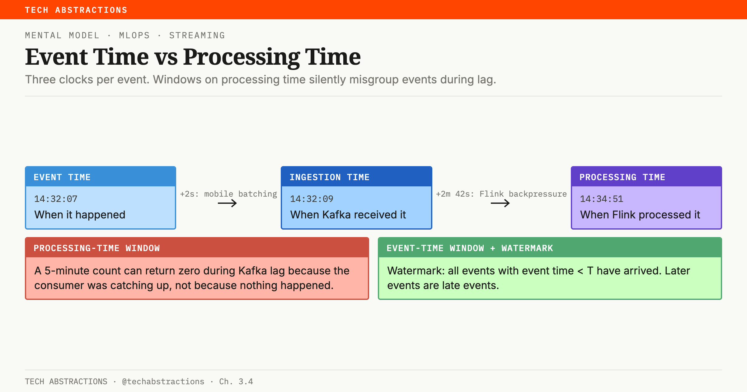
A 5-minute window defined on processing time groups events that occurred at very different actual times. During a Kafka lag event, a "5-minute transaction count" feature computed on processing time can return zero, not because no transactions occurred, but because the consumer was catching up from an earlier backlog.

For training data, this is catastrophic: labels are defined on real-world time (did fraud occur in the next hour?), but features computed on system time do not correspond to the actual state of the world at the labeled time. The model learns to predict from a feature vector that does not reflect reality.

Watermarks solve this. A watermark is a signal that says: "I believe all events with event time < T have arrived." Events arriving after the watermark for their window are "late events." Apache Flink's BoundedOutOfOrdernessWatermarks sets the watermark at max_observed_event_time - out_of_orderness_bound:

class EventTimestampAssigner(TimestampAssigner):
    def extract_timestamp(self, value, record_timestamp):
        return value["event_timestamp_ms"]

watermark_strategy = (
    WatermarkStrategy
    .for_bounded_out_of_orderness(Duration.of_seconds(30))
    .with_timestamp_assigner(EventTimestampAssigner())
)

stream_with_watermarks = env.from_source(kafka_source, watermark_strategy, "kafka")

result = (
    stream_with_watermarks
    .key_by(lambda e: e["user_id"])
    .window(TumblingEventTimeWindows.of(Time.minutes(5)))
    .aggregate(TransactionCountAggregator())
)

Setting the bound to 30 seconds means: wait 30 extra seconds for out-of-order events before closing the window. The tradeoff: a larger bound means fewer missed events but higher feature latency; a smaller bound means lower latency but some late events are dropped or routed to a side output. (Flink also has a separate window-level allowedLateness setting that keeps window state open for very late events; do not confuse the two.)

Point-in-time correctness is the hardest property. Training data must join labels to the feature vector the model would have seen at the label's event timestamp, not features computed at training time. Every ML training pipeline that uses streaming features must query the feature store with event_timestamp, not NOW():

# Point-in-time correct feature retrieval (Feast)
training_df = store.get_historical_features(
    entity_df=labels_df[["user_id", "event_timestamp", "label"]],
    features=[
        "transaction_features:tx_count_5min",
        "transaction_features:tx_amount_avg_1hr",
        "user_features:account_age_days",
    ],
).to_df()
# Each row gets features as of that row's event_timestamp — not today's values

---

Think About It: Setting the watermark for product view events

ShopSense's mobile app batches product view events and flushes them every 15 seconds. The backend API emits events synchronously (< 1 second latency). During peak traffic (flash sales), Kafka consumer lag increases to 2–3 minutes.

You need to set the out-of-orderness bound (the for_bounded_out_of_orderness duration) for the ShopSense product view event stream. Consider:

1. If you set the bound to 5 seconds: what percentage of mobile events might be dropped as late? What latency does this impose on the feature pipeline?
2. If you set the bound to 5 minutes: what is the end-to-end latency from event occurrence to feature available in the online store? Is this acceptable for a real-time recommendation feature?
3. What would you actually set? What monitoring would you add to verify your choice is correct in production?

---

Section 3: Exactly-Once Semantics

"Exactly-once" does not mean an event is processed once. It means the effect of processing each event appears in the output exactly once, even if the event was processed multiple times internally due to failures and retries.

Three delivery guarantees exist:

At-most-once: Messages may be lost but never duplicated. Appropriate for non-critical metrics.

At-least-once: Messages are never lost but may be duplicated. Easy to implement. Requires idempotent downstream consumers.

Exactly-once (effectively-once): Output state reflects exactly one processing of each input event. Requires checkpointing + idempotent or transactional sinks.

Flink implements this via distributed snapshots (the Chandy-Lamport algorithm):

Checkpoint timeline:
  CP1 committed at Kafka offset 10,000
  Events 10,001–11,500 processed
  Job fails at offset 11,501
  Flink restores state to CP1, replays from offset 10,001
  Events 10,001–11,500 re-processed (exactly-once via idempotent Redis sink)

env.enable_checkpointing(60_000)  # 60-second interval
env.get_checkpoint_config().set_checkpointing_mode(CheckpointingMode.EXACTLY_ONCE)
env.get_checkpoint_config().set_min_pause_between_checkpoints(30_000)
env.get_checkpoint_config().set_checkpoint_timeout(120_000)
env.set_state_backend(EmbeddedRocksDBStateBackend(enable_incremental_checkpointing=True))
env.get_checkpoint_config().set_checkpoint_storage(
    FileSystemCheckpointStorage("s3://shopsense-checkpoints/flink/")
)

The practical rule: use exactly-once for COUNT and SUM aggregations where duplicates produce wrong values. For naturally idempotent features (MAX, MIN, LAST_VALUE), at-least-once with idempotent sinks is sufficient and cheaper. Exactly-once imposes I/O overhead. At Netflix's scale (multi-terabyte Flink state), checkpoint duration is a first-order engineering concern.

---

Think About It: Audit your feature aggregations

For each of the following ShopSense streaming feature aggregations, decide: does it require exactly-once semantics, or is at-least-once with an idempotent sink sufficient?

1. user_session_page_count: number of pages viewed in the current session
2. product_max_price_today: maximum listed price for a product across all catalog updates today
3. user_last_purchase_amount: amount of the most recent completed purchase
4. category_purchase_count_7d: total number of purchases in a category over the last 7 days (used for trending calculation)
5. user_tx_velocity_5min: count of transactions in the last 5 minutes (used for fraud scoring)

For the ones that require exactly-once, what breaks if at-least-once is used instead? What is the business impact of the incorrect feature value?

---

VILLAIN CASE STUDY: The Recommendation Engine That Learned From the Future

A mid-sized streaming company built a recommendation engine for "trending content" personalization. The training pipeline joined user interaction events to a "trending score" feature, a 24-hour view count per content item. Training-time AUC: 0.88. An A/B test showed 8% click-through improvement over the baseline. The model was deployed.

Three months after deployment, recommendations for new users (cold-start) were dramatically better than expected, but recommendations for established users had slowly degraded. Churn in the 30–60 day user cohort increased 4%.

The investigation:

# Check: does training data use future-leaked features?
for _, row in training_sample.iterrows():
    historical_score = feature_store.get_historical_features(
        entity_df=pd.DataFrame([{
            "item_id": row["item_id"],
            "event_timestamp": row["event_timestamp"]
        }]),
        features=["trending_features:trending_score_24hr"]
    ).to_df()["trending_score_24hr"].iloc[0]

    training_score = row["trending_score_24hr"]
    shift = abs(historical_score - training_score) / (historical_score + 1e-9)
    if shift > 0.1:
        print(f"LEAKAGE: item {row['item_id']} at {row['event_timestamp']}")

Result: 94% of training rows had temporal leakage. The trending score in the training data reflected the score at training pipeline run time (days after the event), not at event time. The model had learned that "content that would become popular later" drove clicks.

For established users, the model learned to recommend already-popular content (high trending scores at training time). For new users, the cold-start fallback worked correctly. As established users' preferences evolved beyond the popular-at-training-time content, they churned.

The fix: Switch to point-in-time feature retrieval. Add a CI check: for every new training run, sample 1000 rows and compare feature-value-at-event-time vs feature-value-at-training-time. Fail training if more than 10% of sampled rows differ from their event-time value by more than 10%.

Timeline: 3 months of degraded recommendations. 4 days to identify root cause. Estimated revenue impact: $1.2M in churn-attributed losses.

The lesson: Temporal leakage is invisible in offline metrics; it inflates them. The signal is a gap between offline AUC and online CTR that cannot be explained by distribution shift. Prevention requires point-in-time correctness enforced in CI, not on an honor system.

---

Section 4: Streaming Pipeline Architecture

A production streaming ML pipeline has five layers:

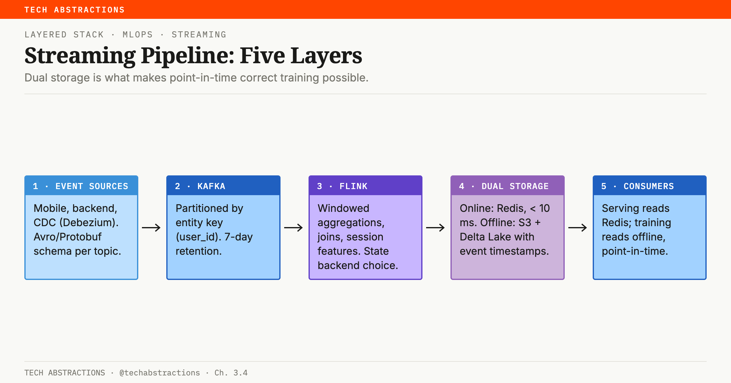
Layer 1 (Event sources): Mobile apps, backend services, CDC (Debezium for database row changes). Each publishes to Kafka with a registered Avro/Protobuf schema. Schema enforcement at ingest prevents downstream processing failures from silent field changes.

{
  "type": "record",
  "name": "ProductViewEvent",
  "namespace": "com.shopsense.events.v1",
  "fields": [
    {"name": "event_id", "type": "string"},
    {"name": "user_id", "type": "string"},
    {"name": "product_id", "type": "string"},
    {"name": "event_timestamp_ms", "type": "long"},
    {"name": "session_id", "type": "string"},
    {"name": "price_at_view", "type": ["null", "double"], "default": null}
  ]
}

Layer 2 (Kafka transport): Partitioned by entity key (user_id for user features). This keeps each user's events in order within one partition, and Flink's key_by routes every event for a user to the same task, enabling stateful aggregations without distributed joins. Retention: 7 days, enabling short-window replay.

Layer 3 (Flink processing): Windowed aggregations, joins, session features. Key decision: state backend. HashMapStateBackend for small-state jobs; EmbeddedRocksDBStateBackend for large-state (Netflix has reported jobs with multi-terabyte state). Hot-key skew (celebrity/bot users) handled via key salting or pre-aggregation.

Layer 4 (Dual storage): Online store (Redis) for < 10ms serving; offline store (S3 + Delta Lake) with event timestamps for training and backfill. The dual write is what makes point-in-time correct training possible.

Layer 5 (Consumers): Online serving reads from Redis on every inference request. Training pipelines read from the offline store with point-in-time queries.

---

Section 5: Lambda vs Kappa Architecture

Two patterns dominate ML data systems. The choice has long-term maintenance consequences.

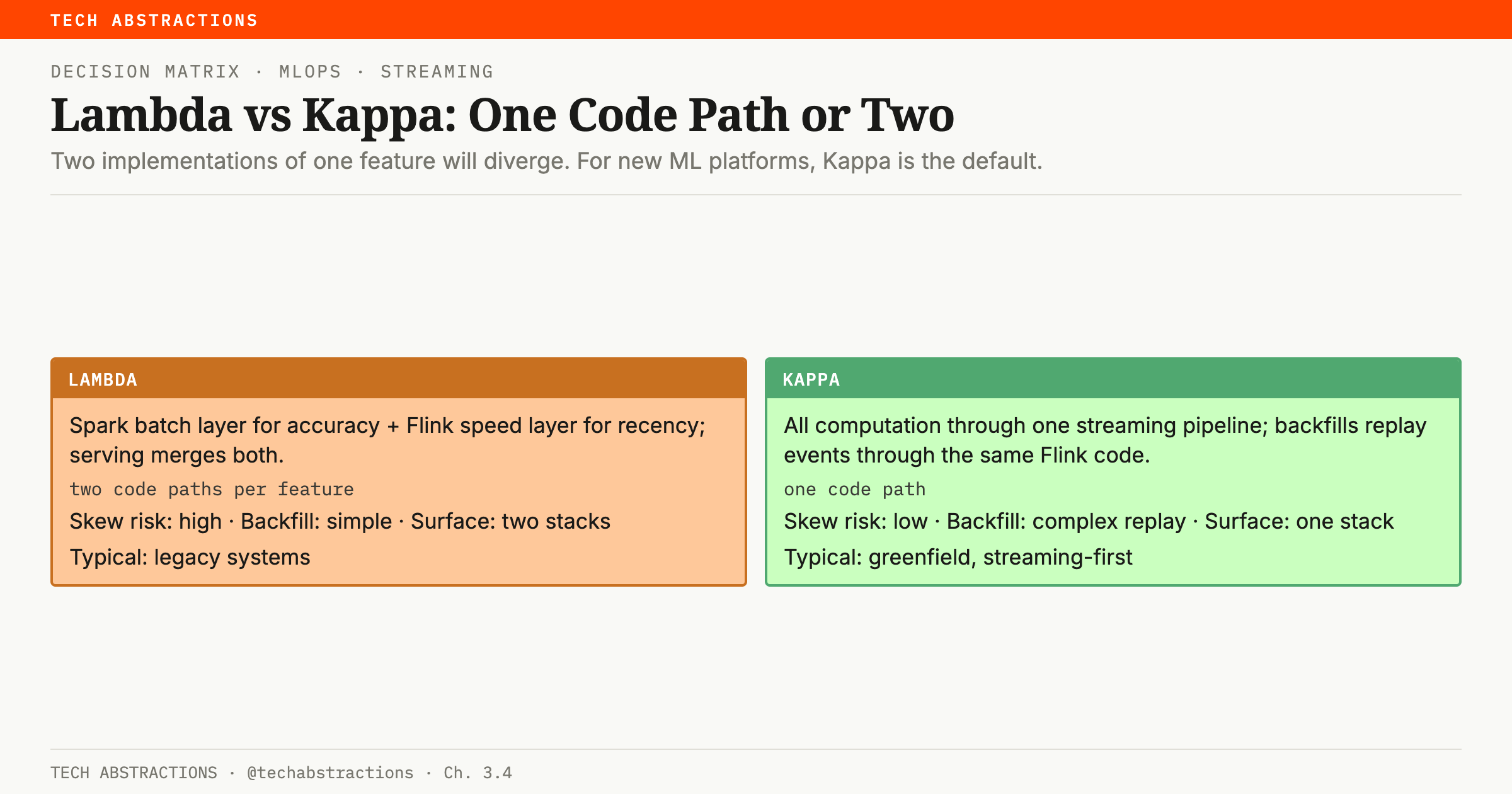
Lambda maintains two processing paths: a Spark batch layer for historical accuracy and a Flink speed layer for recency. The serving layer merges both.

The fundamental problem: two code paths for the same feature logic. A "7-day purchase count" has a Spark implementation and a Flink implementation. They will diverge: different null handling, different timestamp semantics, different edge cases. Training-serving skew is baked into the architecture.

Kappa eliminates the batch layer. All computation runs through the same streaming pipeline. Historical backfills replay events through the same Flink code. One code path. The cost: complex replay for long historical windows.

Uber's "Kappa+" runs the same FlinkSQL on both Kafka (real-time) and Hive (batch backfill). Single codebase, Spark-like throughput for large historical windows.

Criterion	Lambda	Kappa
Training-serving skew risk	High (two code paths)	Low (one code path)
Backfill simplicity	Simple (Spark batch)	Complex (bounded streaming replay)
Operational surface	Large (two stacks)	Smaller (one stack)
Typical use case	Legacy systems	Greenfield, streaming-first

For new ML platforms, Kappa is the default. Lambda only when existing batch infrastructure is too expensive to replace and the team has exceptional discipline to keep two code paths synchronized.

---

Section 6: Backfill and Replay

Streaming backfill (adding a new feature retroactively, fixing a pipeline bug, recovering from an outage) is harder than batch because Kafka retention is limited (7 days), Flink needs modification for bounded historical input, and replay must preserve event-time semantics.

Kafka replay (< 7 days): Start a separate job from the desired Kafka offset, with fresh state and offline-only output. Same Flink code. Fast and simple. (Restoring the live job's state and replaying on top of it would double-count.)

Re-ingestion from object storage: Raw events logged to S3 → re-ingest into a backfill Kafka topic → same Flink job with backfill source → write only to offline store (not production online store).

Spark-based recomputation: For features without streaming semantics requirements. Simpler, but reintroduces Lambda code-path divergence.

DoorDash Riviera's team documented that treating backfill as a first-class concept changed feature pipeline design: every feature definition specifies its backfill strategy at design time. The operational cost of discovering a missing backfill strategy during a production incident far exceeds the cost of specifying it upfront.

The critical constraint: backfilled features must be point-in-time correct. A feature backfilled on February 1 for events that occurred on January 15 must reflect the state of the world on January 15. This requires:

1. Event timestamps (not system timestamps) for all time-based computations
2. Writing records with original event timestamps to the offline store
3. Not overwriting production online store values (backfill to offline only)

---

Section 7: Feature Freshness and Training-Serving Skew

Feature freshness is not just an SLA; it is a model correctness property. Stale features produce systematic bias, not random noise.

LinkedIn reported that recommendation model ROC-AUC falls steadily as feature delay grows: about 4.5% lower at a 24-hour delay than at a 1-minute delay. Fraud models with velocity features are far more delay-sensitive.

Reported freshness targets (vendor-stated, not independently verified):

• LinkedIn near-real-time features: < 15 seconds event-to-serving
• Tecton production platform: < 1 second (real-time), < 15 seconds (streaming)
• DoorDash delivery-time features: < 5 seconds
• Uber surge pricing: sub-second (event-driven)

Training-serving skew in streaming systems has five root causes:

1. Different code paths: Spark (training) and Flink (serving) implementations of the same feature diverge. Solution: feature store that executes the same transformation in both paths.
2. Temporal leakage: Training labels joined to feature values at training time, not at event time.
3. Feature unavailability: A feature was available during training but the serving system returns null at 3 AM when the batch job hasn't run. Silent, systematic degradation.
4. Backfill inconsistency: Spark-backfilled training data differs subtly from live Flink-computed values.
5. Distribution shift: Training data from 6 months ago has different distribution than the live stream.

def detect_feature_skew(training_values: list, serving_values: list,
                         feature_name: str, alpha: float = 0.05) -> dict:
    ks_stat, p_value = stats.ks_2samp(training_values, serving_values)
    training_mean = pd.Series(training_values).mean()
    serving_mean = pd.Series(serving_values).mean()
    mean_shift_pct = abs(serving_mean - training_mean) / (training_mean + 1e-9)
    return {
        "feature": feature_name,
        "ks_statistic": round(ks_stat, 4),
        "p_value": round(p_value, 4),
        "significant_skew": p_value < alpha,
        "mean_shift_pct": round(mean_shift_pct * 100, 2),
        "recommendation": "investigate" if p_value < alpha else "ok"
    }

---

Section 8: Tiled Window Aggregations

Long-window features (7-day counts, 30-day averages) with sub-second freshness cannot be handled naively. Keeping 7 days of raw events in Flink state for 10M users requires 500+ GB of keyed state.

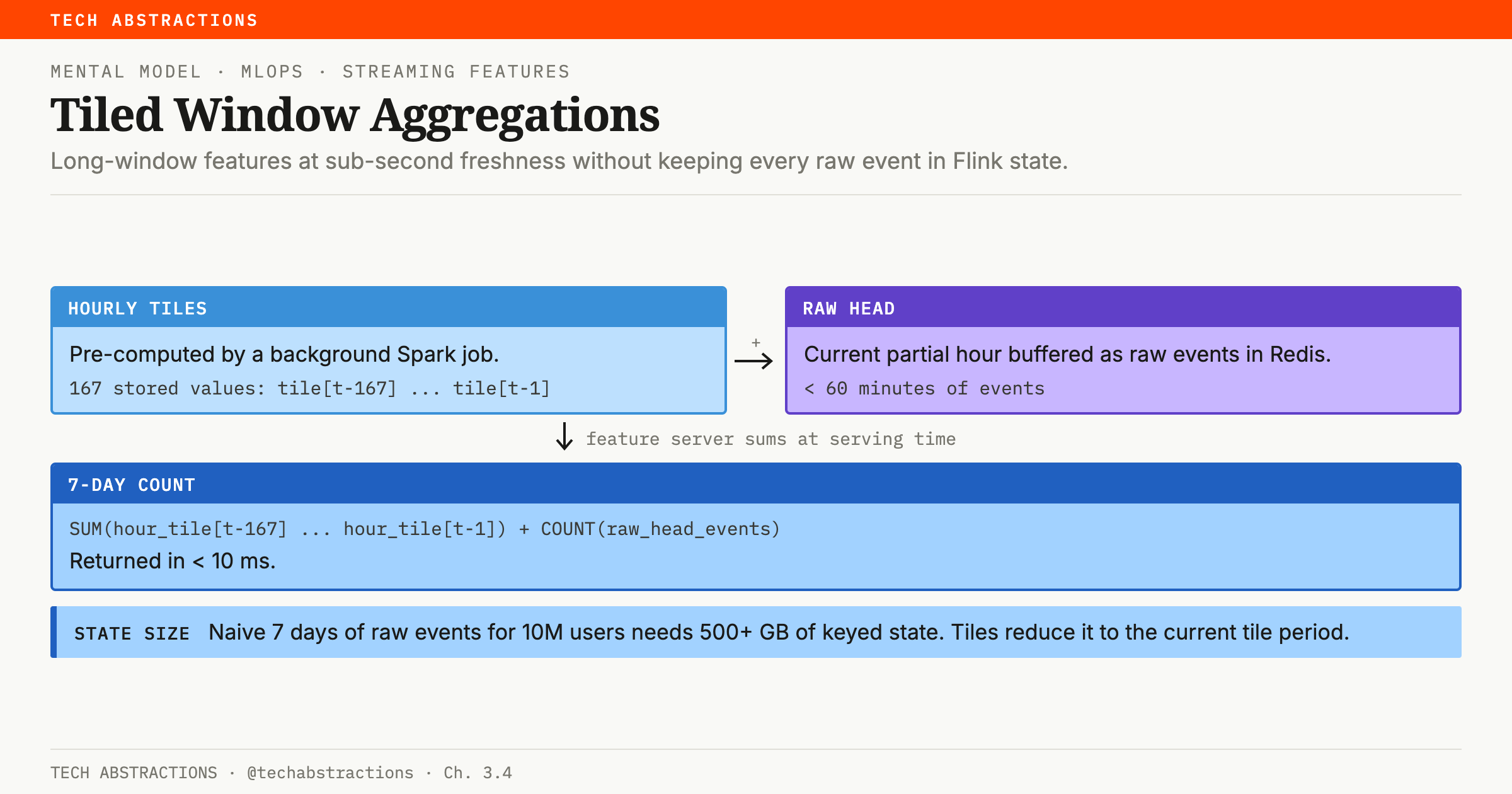
The tiled approach (Tecton, similar to Airbnb Sawtooth Windows): pre-compute hourly tile aggregations via a background Spark job, buffer the current partial hour as raw events in Redis, and at serving time assemble by summing tiles + raw head:

7-day count = SUM(hour_tile[t-167] ... hour_tile[t-1]) + COUNT(raw_head_events)

The feature server reads 167 stored values plus < 60 minutes of raw events and returns the result in < 10ms. Flink state drops from O(all events in window) to O(raw events in the current tile period).

The same tile structure enables point-in-time correct training: the offline store holds the same tiles and raw event logs. The training pipeline reads from the offline store to reconstruct any historical feature value.

---

CASE STUDY (Free): DoorDash Riviera: Declarative Streaming at Scale

DoorDash's Riviera platform is a declarative framework for Flink-based streaming feature pipelines. At publication, it powered real-time features for delivery-time estimation, dasher matching, and fraud detection, processing billions of events daily.

Decision 1: Declarative YAML over Flink code

Riviera lets users define streaming feature pipelines declaratively on top of Flink. The YAML below is an illustrative sketch of that style, not DoorDash's published syntax:

feature_pipeline:
  name: user_transaction_velocity
  source:
    topic: transaction_events
    schema: com.shopsense.events.v1.TransactionEvent
    watermark_strategy: bounded_out_of_orderness
    max_out_of_orderness_seconds: 30
  transformations:
    - type: filter
      condition: "amount > 0 AND status = 'COMPLETED'"
    - type: window_aggregate
      group_by: [user_id]
      window: tumbling_5min
      aggregations:
        - field: transaction_id
          function: COUNT
          output_name: tx_count_5min
        - field: amount
          function: SUM
          output_name: tx_amount_sum_5min
  sinks:
    - type: redis
      key_pattern: "user:{user_id}:velocity"
      ttl_seconds: 3600
    - type: delta_lake
      path: s3://features/transaction_velocity/
      partition_by: event_date

Why it worked: Most streaming feature pipelines share the same structural patterns. Requiring engineers to write raw Flink Java for each created 100+ custom, independently maintained codebases. YAML declarations reduced pipeline creation time from weeks to hours and made it accessible to ML engineers without Flink expertise.

Decision 2: Backfill as a first-class concept

Every Riviera feature definition includes a backfill_strategy block specifying source, maximum backfill window, and whether backfill writes to online store (typically no). Backfill became a standard operation rather than a fire-drill. Engineers could run riviera backfill --feature user_transaction_velocity --from 2024-01-01 and the platform handled bounded Flink execution against historical Hive data.

Decision 3: Schema enforcement at job startup

Riviera validates the Kafka message schema against the Schema Registry at job startup. If the schema has changed incompatibly (field renamed, type widened), the job fails immediately with a clear error, not silently producing null features at runtime. Most schema drift incidents are caught within minutes of a schema change being deployed, before they reach model serving.

Decision 4: Single Flink runtime for 100+ pipelines

Rather than a separate Flink cluster per pipeline, Riviera deploys one generalized Flink JAR parameterized by YAML. Upgrades, monitoring, and debugging happen in one place. The tradeoff: a runtime bug affects all pipelines simultaneously. DoorDash mitigated this with canary deployments of runtime upgrades to a pipeline subset before full rollout.

The core lesson: The organizational challenge of streaming feature pipelines is not the Flink engineering. It is the proliferation of one-off, hard-to-operate pipelines that accumulate over time. Declarative platforms succeed not because YAML is powerful but because they force standardization and create a single operational surface.

---

Advanced Exercise 1: Streaming vs Batch Feature Classification

Context: ShopSense is designing the feature set for the next version of its recommendation engine. The following 8 features are under consideration. Your task is to classify each and design its implementation.

For each feature, provide:

1. Freshness class (historical / batch-fresh / near-real-time / real-time)
2. Justified streaming vs batch decision (with freshness-accuracy reasoning)
3. If streaming: window type and size, watermark strategy, exactly-once vs at-least-once
4. If batch: schedule, storage format, staleness upper bound

Features:

1. user_lifetime_purchase_count: total purchases since account creation
2. product_view_count_last_2hr: number of users who viewed a product in the last 2 hours (used for trending)
3. user_preferred_brands_90d: user's top 5 brands by purchase frequency, last 90 days
4. user_session_view_count: number of product views in the current active session
5. category_conversion_rate_7d: purchase/view ratio per category, last 7 days
6. user_tx_velocity_5min: transaction count in last 5 minutes (fraud feature)
7. product_price_change_indicator: flag set when a product's price dropped > 10% in the last hour
8. user_cart_abandonment_rate_30d: fraction of carts not converted, last 30 days

Deliverable: A feature classification table with implementation justification for each row. For streaming features, include a Flink window configuration snippet.

---

Advanced Exercise 2: Temporal Leakage Diagnosis

Scenario: You are reviewing a colleague's training pipeline for a ShopSense demand forecasting model. The model predicts the probability that a product will be out-of-stock in the next 24 hours. Offline AUC is 0.92, but online precision@K is significantly lower than expected from offline evaluation.

You suspect temporal leakage. Here is the relevant training data assembly code:

def build_training_dataset(events_df: pd.DataFrame, 
                            labels_df: pd.DataFrame) -> pd.DataFrame:
    # Get current feature values for all products in the training set
    product_ids = labels_df["product_id"].unique().tolist()
    
    # Fetch current inventory features
    inventory_features = feature_store.get_online_features(
        features=[
            "inventory_features:current_stock_level",
            "inventory_features:reorder_velocity_7d",
            "inventory_features:supplier_lead_time_days",
            "inventory_features:sales_velocity_24hr",
        ],
        entity_rows=[{"product_id": pid} for pid in product_ids]
    ).to_df()
    
    # Join labels to features
    training_df = labels_df.merge(
        inventory_features, on="product_id", how="left"
    )
    
    # Add event-level features
    event_features = events_df.groupby("product_id").agg({
        "purchase_amount": ["mean", "sum"],
        "view_count": "sum"
    }).reset_index()
    
    return training_df.merge(event_features, on="product_id", how="left")

Your tasks:

1. Identify every source of temporal leakage in this code. Be specific: which line, which feature, why it constitutes leakage.
2. For each identified leakage, estimate the direction and magnitude of the resulting bias (does it inflate or deflate offline AUC?).
3. Write the corrected version of build_training_dataset() using point-in-time correct feature retrieval.
4. Design a temporal leakage CI check that could be added to the training pipeline to automatically detect this class of error.

---

Advanced Exercise 3: Watermark Calibration Analysis

Scenario: ShopSense has deployed a Flink job computing user_session_view_count, the number of product views in the current 30-minute tumbling window. The job uses an out-of-orderness bound of 15 seconds.

During a post-incident review, you discover:

• 8% of mobile app events arrive 20–45 seconds after their event timestamp (mobile batching)
• 2% of events arrive 60–180 seconds late (poor connectivity users on mobile data)
• 0.3% of events arrive > 5 minutes late (background sync from offline mode)
• The recommendation model uses this feature to detect "active session" users (defined as > 3 views in the window)

Your tasks:

1. Estimate the false negative rate for "active session" detection given the current 15-second watermark. Which user cohorts are most affected?
2. Calculate the end-to-end feature latency (event occurrence → feature available in online store) for three watermark settings: 15s, 60s, 3 minutes.
3. Recommend a watermark setting and justify it using the business cost of false negatives vs latency tradeoff.
4. Design a side output handler for late events that arrives > 3 minutes late. What should be done with these events? (Options: drop, recompute window, emit correction to online store, log to monitoring only.)

---

Real-World Implementation 1: Flink Streaming Feature Pipeline

Task: Build a production-ready Flink streaming feature pipeline for ShopSense transaction velocity features.

Scaffold to implement:

# shopsense_streaming_features/transaction_velocity_pipeline.py
from pyflink.datastream import StreamExecutionEnvironment, CheckpointingMode
from pyflink.datastream.connectors.kafka import KafkaSource, KafkaOffsetsInitializer
from pyflink.datastream.window import TumblingEventTimeWindows
from pyflink.common import WatermarkStrategy, Duration, Time
from pyflink.common.watermark_strategy import TimestampAssigner
from pyflink.datastream.state import ValueStateDescriptor
from pyflink.datastream.functions import AggregateFunction
import redis
import json


class TransactionEvent:
    """Parsed transaction event with event-time semantics."""
    def __init__(self, user_id: str, transaction_id: str, amount: float,
                 status: str, event_timestamp_ms: int):
        self.user_id = user_id
        self.transaction_id = transaction_id
        self.amount = amount
        self.status = status
        self.event_timestamp_ms = event_timestamp_ms


class VelocityAggregator(AggregateFunction):
    """
    Aggregate: count and sum of completed transactions in window.
    Must handle exactly-once (COUNT is not idempotent).
    """
    def create_accumulator(self):
        # TODO: return initial accumulator state (count=0, amount_sum=0.0)
        pass

    def add(self, value: TransactionEvent, accumulator):
        # TODO: update accumulator with new event (filter status='COMPLETED')
        # and return the updated accumulator (the tests below use the return value)
        pass

    def get_result(self, accumulator) -> dict:
        # TODO: return {"tx_count": int, "tx_amount_sum": float}
        pass

    def merge(self, acc1, acc2):
        # TODO: merge two accumulators (for session windows)
        pass


class DualWriteSink:
    """
    Write velocity features to Redis (online serving) and
    emit records for Delta Lake offline store (via Kafka sink topic).
    """
    def __init__(self, redis_host: str, redis_port: int = 6379):
        self.redis_host = redis_host
        self.redis_port = redis_port
        self._redis_client = None

    def _get_redis(self):
        if self._redis_client is None:
            self._redis_client = redis.Redis(
                host=self.redis_host, port=self.redis_port,
                decode_responses=True
            )
        return self._redis_client

    def write_online(self, user_id: str, window_start_ms: int,
                     tx_count: int, tx_amount_sum: float,
                     ttl_seconds: int = 3600):
        # TODO: write to Redis with key pattern "user:{user_id}:tx_velocity:5min"
        # Store as hash: {"count": tx_count, "amount_sum": tx_amount_sum,
        #                  "window_start": window_start_ms, "updated_at": now}
        pass

    def write_offline_record(self, record: dict) -> dict:
        # TODO: return a record dict for offline Delta Lake logging
        # Must include: user_id, window_start_ms, window_end_ms,
        #               tx_count, tx_amount_sum, computed_at_ms
        pass


def build_velocity_pipeline(
    kafka_bootstrap_servers: str,
    kafka_topic: str,
    redis_host: str,
    window_minutes: int = 5,
    max_out_of_orderness_seconds: int = 30,
    checkpoint_interval_ms: int = 60_000,
) -> StreamExecutionEnvironment:
    """
    Build and return a configured Flink StreamExecutionEnvironment
    for transaction velocity feature computation.
    
    Pipeline: Kafka → parse → filter COMPLETED → watermark → 
              5-min tumbling window → aggregate → DualWriteSink
    """
    env = StreamExecutionEnvironment.get_execution_environment()
    
    # TODO 1: Configure checkpointing (exactly-once, 60s interval,
    #          30s min pause, RocksDB state backend, S3 checkpoint storage)
    
    # TODO 2: Configure Kafka source with:
    #   - EARLIEST offset for new jobs (or COMMITTED for restarts)
    #   - Bounded out-of-orderness watermark strategy using event_timestamp_ms field
    #   - max_out_of_orderness_seconds parameter

    # TODO 3: Build the pipeline:
    #   - Parse JSON → TransactionEvent (handle malformed records → DLQ side output)
    #   - Filter: status == 'COMPLETED' and amount > 0
    #   - Key by user_id
    #   - Apply tumbling event-time window of window_minutes
    #   - Aggregate with VelocityAggregator
    #   - Sink to DualWriteSink (online Redis + offline record emission)

    return env


def run_backfill(
    s3_historical_path: str,
    start_date: str,
    end_date: str,
    redis_host: str,
    write_online: bool = False,  # False for backfill — offline only
) -> None:
    """
    Backfill transaction velocity features from S3 historical event logs.
    Uses bounded source; same aggregation logic as live pipeline.
    """
    # TODO: implement using Flink FileSource (bounded) reading Parquet from S3
    # Key difference from live pipeline:
    #   1. Source is FileSource, not KafkaSource
    #   2. write_online=False: skip Redis write, write offline record only
    #   3. Job terminates when source is exhausted (bounded input)
    pass

Implementation requirements:

1. VelocityAggregator: implement all four methods. add() must be idempotent-safe given exactly-once guarantees.
2. DualWriteSink.write_online(): use Redis HSET with TTL. Include window_start_ms in the stored hash for debugging.
3. build_velocity_pipeline(): configure checkpointing correctly, configure watermark with the event_timestamp_ms field from the JSON payload, handle malformed records via side output to a dead_letter topic.
4. run_backfill(): implement using Flink's bounded FileSource reading the historical Parquet files. Must not write to Redis online store.

Test to pass:

def test_velocity_aggregator_exactly_once():
    agg = VelocityAggregator()
    acc = agg.create_accumulator()
    
    # Process 3 events
    for i in range(3):
        event = TransactionEvent(
            user_id="u1", transaction_id=f"tx{i}",
            amount=10.0 + i, status="COMPLETED",
            event_timestamp_ms=1700000000000 + i * 1000
        )
        acc = agg.add(event, acc)
    
    result = agg.get_result(acc)
    assert result["tx_count"] == 3
    assert abs(result["tx_amount_sum"] - 33.0) < 0.001

def test_aggregator_filters_non_completed():
    agg = VelocityAggregator()
    acc = agg.create_accumulator()
    
    events = [
        TransactionEvent("u1", "tx1", 50.0, "COMPLETED", 1700000000000),
        TransactionEvent("u1", "tx2", 30.0, "PENDING", 1700000001000),
        TransactionEvent("u1", "tx3", 20.0, "FAILED", 1700000002000),
    ]
    for e in events:
        acc = agg.add(e, acc)
    
    result = agg.get_result(acc)
    assert result["tx_count"] == 1
    assert abs(result["tx_amount_sum"] - 50.0) < 0.001

---

Real-World Implementation 2: Point-in-Time Correctness Validator

Task: Build a CI tool that validates point-in-time correctness for any training dataset.

Scaffold:

# shopsense_mlops/pit_correctness_validator.py
import pandas as pd
import numpy as np
from dataclasses import dataclass
from typing import Optional
from feast import FeatureStore


@dataclass
class SkewReport:
    feature_name: str
    sample_size: int
    pct_rows_with_skew: float        # fraction with > threshold_pct shift
    mean_absolute_shift_pct: float   # average shift across all rows
    max_shift_pct: float             # worst-case row
    has_temporal_leakage: bool       # True if pct_rows_with_skew > leakage_threshold
    direction: str                   # "inflated" | "deflated" | "mixed" | "clean"
    p_value: float                   # KS test p-value


def sample_training_dataset(
    training_df: pd.DataFrame,
    n_samples: int = 1000,
    random_state: int = 42
) -> pd.DataFrame:
    """Sample rows for validation. Preserves temporal distribution."""
    # TODO: stratified sample by date (to avoid over-sampling recent data)
    # Return sample with columns: entity_id, event_timestamp, feature_name, training_value
    pass


def query_historical_features(
    sample_df: pd.DataFrame,
    feature_store: FeatureStore,
    feature_refs: list[str],
) -> pd.DataFrame:
    """
    Query feature store for historical values at each row's event_timestamp.
    Returns sample_df with additional columns: {feature_name}_historical
    """
    # TODO: use feature_store.get_historical_features() with entity_df
    # entity_df must have: entity_id column + event_timestamp column
    # Merge historical values back to sample_df
    pass


def compute_skew_report(
    sample_df: pd.DataFrame,
    feature_name: str,
    training_col: str,
    historical_col: str,
    shift_threshold_pct: float = 0.10,
    leakage_threshold: float = 0.10,
) -> SkewReport:
    """
    Compare training values to point-in-time historical values.
    
    A positive mean shift (training > historical) indicates temporal leakage:
    the model was trained on values that reflect future state.
    """
    # TODO: compute shift per row: |training - historical| / (|historical| + 1e-9)
    # Determine direction: if training_mean > historical_mean → inflated (likely leakage)
    # Run KS test between training values and historical values
    # Return SkewReport dataclass
    pass


def validate_training_dataset(
    training_df: pd.DataFrame,
    feature_store: FeatureStore,
    feature_refs: list[str],
    entity_col: str,
    timestamp_col: str,
    n_samples: int = 1000,
    fail_on_leakage: bool = True,
) -> tuple[bool, list[SkewReport]]:
    """
    Run full point-in-time correctness validation.
    
    Returns (passed, reports). If fail_on_leakage=True and any feature
    has has_temporal_leakage=True, raises ValueError with a summary report.
    
    Usage in training pipeline:
        passed, reports = validate_training_dataset(
            training_df=df,
            feature_store=store,
            feature_refs=["tx_features:tx_count_5min", "tx_features:tx_amount_avg"],
            entity_col="user_id",
            timestamp_col="event_timestamp",
        )
    """
    # TODO: orchestrate sample → query → compute_skew_report for each feature
    # Print a summary table (feature | pct_skewed | mean_shift | leakage?)
    # Raise ValueError if fail_on_leakage=True and any report.has_temporal_leakage=True
    pass


# pytest test
def test_clean_dataset_passes_validation():
    """Training data with correct point-in-time retrieval should pass."""
    # Build a synthetic training dataset where training values == historical values
    # (no leakage). validate_training_dataset should return passed=True.
    pass

def test_leaked_dataset_fails_validation():
    """Training data with future-leaked features should fail validation."""
    # Build synthetic training dataset where training values reflect future state.
    # validate_training_dataset should return passed=False and
    # the leaking feature's SkewReport.has_temporal_leakage should be True.
    pass

Implementation requirements:

1. sample_training_dataset(): stratified by event_timestamp.dt.date; sample proportionally from each date to avoid over-representing recent data.
2. compute_skew_report(): direction detection: if training_mean > historical_mean by > threshold, classify as "inflated" (most likely temporal leakage); if training_mean < historical_mean, "deflated" (possible feature freshness issue at serving time).
3. validate_training_dataset(): print a formatted summary table; the raised ValueError must include the feature name, pct_skewed, and mean_shift_pct to make the error actionable.

---

Production Challenge 1: Streaming Pipeline Cascade Failure

Scenario: ShopSense's Kafka consumer lag monitor fires at 3:47 AM on a Tuesday. The transaction_events topic has 8 million unprocessed messages (normally < 50,000). The Flink job is running but processing at 10% of normal throughput.

Investigation reveals:

• A new product category was added at 3:12 AM, and products were bulk-ingested, 500,000 product_catalog_update events in 8 minutes
• The Flink job performs a stream-stream join: transaction_events JOIN product_catalog_updates ON product_id with a 30-minute event-time window
• The stream-stream join maintains state for all unmatched events within the join window
• The 500,000 catalog updates are all for products from a single new category: category_id = "FLASH_SALE_ELECTRONICS"
• The fraud scoring model is using stale features during this period
• The recommendation model is receiving null for the product_category feature for all transactions in the last 40 minutes

Your tasks:

1. Diagnose the root cause precisely. What is happening in the Flink job state? Why is throughput degraded by 90%?
2. Immediate remediation: what action do you take right now to restore fraud scoring to working state?
3. Architectural fix: how do you redesign the stream-stream join to prevent this from happening again?
4. Monitoring design: what alert should have fired before the 3:47 AM cascade failure? What metric, what threshold, what lead time?
5. Null-feature handling: the recommendation model received null product_category for 40 minutes. What should a well-designed serving system do when a streaming feature is null due to pipeline lag? Design the fallback policy.

---

Production Challenge 2: Training-Serving Skew Post-Deployment Investigation

Scenario: ShopSense deployed a new fraud detection model 6 weeks ago. Offline AUC was 0.91. Online precision is 0.73 (vs 0.79 for the previous model). The model is flagging 40% more transactions as potentially fraudulent, but the false positive rate is higher than expected.

Feature analysis shows:

• tx_velocity_5min (streaming): online serving mean = 1.8, training distribution mean = 3.4
• user_account_age_days (batch): online serving mean = 187, training distribution mean = 187 (✓)
• tx_amount_avg_1hr (streaming): online serving mean = $47.20, training distribution mean = $89.40

Your tasks:

1. Given the feature distribution data, formulate three hypotheses for why tx_velocity_5min shows a 1.6× mean difference between training and serving.
2. Design a diagnostic query to determine which hypothesis is correct. What data do you need, and where would you find it?
3. The tx_amount_avg_1hr shows a 1.9× difference. What is the most likely cause, and how does this differ from the likely cause of the tx_velocity_5min skew?
4. Write a post-incident retrospective section: "What we would do differently in the training pipeline design to catch this before deployment." Include at least 3 concrete process changes.
5. Immediate action: the model is live and producing high false positives. Do you roll back immediately, or keep it running? Justify your decision using a risk framework (false positive cost vs rollback cost vs investigation time).

---

Interview Question 1: Streaming vs Batch: The Architectural Decision

Question (as asked at senior/staff ML engineer interviews):

"We're building a real-time recommendation engine for a flash sale feature that runs for 4 hours, twice per week. During a flash sale, product popularity changes every 5 minutes. Outside flash sales, recommendations are weekly-refresh batch predictions. How would you architect the data pipeline for the trending features? Walk me through your reasoning."

Model answer structure:

Address the key dimensions in order:

1. Freshness requirement analysis. During flash sales, a product's trending score from 5 minutes ago is significantly stale: a product going viral in the last 5 minutes won't surface without near-real-time data. Outside flash sales, weekly-refresh batch is appropriate. The feature has two modes.

2. Architecture recommendation. A hybrid: maintain a streaming pipeline for trending features that runs 24/7 (not just during flash sales), but the batch pipeline writes to a different feature key prefix. The recommendation engine uses the streaming score when freshness is < 10 minutes; falls back to the batch score when streaming is unavailable.

3. Streaming tax justification. A 4-hour event window that is critical to the business justifies streaming infrastructure. The incremental cost of running Flink continuously for this feature set is low relative to the business value. The alternative (spinning up streaming infrastructure only during flash sales) has higher operational risk and cold-start latency.

4. Event-time semantics. Trending score is a COUNT of views. It must be computed over event-time windows. A processing-time window during a spike would produce incorrect counts if Kafka lag increases. Watermark: 30 seconds (product catalog pages are primarily desktop/fast connections).

5. Training data implications. The training pipeline must use point-in-time correct features for flash sale labels, the feature value at the time of the interaction, not the final trending score after the sale ended (which would be the maximum, constituting temporal leakage).

6. Monitoring. Feature freshness SLA: < 30 seconds event-to-serving during flash sales. Alert if freshness degrades > 2 minutes.

---

Interview Question 2: Debugging a Silent Streaming Failure

Question: "Your fraud model's precision has dropped 15% over the last 3 days. The Flink job shows no errors. Kafka consumer lag is normal (< 10,000). Feature freshness monitoring shows < 15 seconds. Walk me through your debugging process."

Model answer structure:

The key insight: all the streaming infrastructure metrics are healthy, which means the failure is likely in feature correctness (wrong values, not missing values) or model distribution shift.

Step 1: Disambiguate pipeline vs model. Pull a sample of recent fraud detections and compare feature values in the model log to what the feature store says those values should be. If they match, the pipeline is correct; the issue is model quality. If they differ, the pipeline is producing wrong values.

Step 2: If pipeline is producing wrong values. Check for recent deployments or schema changes in the last 3 days. A type change in an upstream event (int → float, or a null handling change) can silently alter aggregation values without causing errors. Check the Schema Registry for recent schema version changes.

Step 3: Temporal analysis. When exactly did precision start dropping? If it correlates with a deployment, that's the culprit. If it correlates with a gradual drift, it's more likely distribution shift.

Step 4: Feature distribution comparison. Run detect_feature_skew() comparing the last 3 days of serving feature values to the training distribution. A 1.5× shift in tx_velocity_5min or tx_amount_avg_1hr with no error logs suggests a silent schema change or windowing change.

Step 5: Verify exactly-once. Check checkpoint success metrics. If checkpoints have been failing or taking longer than the checkpoint interval, exactly-once guarantees are void: COUNT aggregations may be double-counting after job restarts.

Output: "My hypothesis is X. Here is the query/check that would confirm or refute it. If confirmed, the fix is Y. If not, my next hypothesis is Z."

---

Interview Question 3: Designing Feature Freshness SLAs

Question: "You're the tech lead for a new streaming ML platform at a mid-size fintech. You need to define feature freshness SLAs for the platform. How do you approach it, and what SLAs would you propose?"

Model answer structure:

Start with business impact, not technology capability. For each feature type, ask: what is the cost of a feature being X minutes stale? For fraud detection velocity features, a 5-minute stale feature can miss 40+ micro-transactions in a velocity attack (direct financial loss). For recommendation trending features, a 30-minute stale feature produces suboptimal recommendations (lower CTR, bounded revenue impact). For user preference features (batch), daily freshness is sufficient.

Differentiate SLA tiers:

• Real-time (fraud, high-stakes): event-to-serving < 10 seconds. Requires streaming compute, Redis online store.
• Near-real-time (recommendations, session): event-to-serving < 60 seconds. Streaming compute, Redis or Cassandra.
• Batch-fresh (user profiles, long-term preferences): updated within 2 hours of batch job completion. Nightly batch, offline feature store.
• Historical (demographics, account metadata): weekly refresh acceptable. Pure batch.

Translate SLAs to architecture requirements:

• < 10 seconds requires Kafka → Flink with short checkpoint intervals (30s), Redis with < 5ms get latency, direct serving path
• < 60 seconds can tolerate 60s checkpoint intervals, allows for Cassandra (higher latency but cheaper at scale)

• 5 minutes can be handled with micro-batch (Spark Structured Streaming with 5-minute trigger)

Monitoring: For each SLA tier, define a P95 freshness metric and a breach SLA threshold. Alert at 2× SLA for investigation, page at 5× SLA for immediate response.

The trap to avoid: Don't define SLAs in terms of what the infrastructure can do today. Define them in terms of what the business needs, then design the infrastructure to meet them. Teams that do it backwards end up with SLAs that are technically achievable but commercially meaningless.