Data Sourcing, Discovery & Understanding
Write the data requirements document before touching a dataset — teams that start with data hunting instead of data specification build models on signals that don't exist at serving time, labels that leak from the future, and sources they'll never be able to audit or trust.
Requirements Before Data: How Production ML Teams Source, Understand, and Trust Their Data
"Bad models are usually bad data decisions with good training code."
Bad models are often just bad data decisions with good training code. The failure mode is predictable: engineers open a data warehouse, find something that looks useful, and start building a feature pipeline. Three months later, the model deploys to production, performs worse than offline metrics predicted, and no one can explain why.
The root cause is almost always one of four things: features that were available during training but not at serving time (training-serving skew), labels that were inadvertently computed using information from the future (temporal leakage), a data source whose distribution doesn't match the population the model will operate on (representation bias), or a pipeline whose upstream source changes without warning (schema drift).
All four failures are preventable. They require specifying data requirements before hunting for data sources, treating data sourcing as an engineering discipline with acceptance criteria, not a discovery process with no definition of done.
This chapter gives you a requirements-first approach to data sourcing. By the end, you'll have a systematic method for specifying what you need before you search, evaluating what you find against those requirements, documenting it in a form that scales across a team, and instrumenting it so failures don't surprise you six months after launch.
The Data Shopping List: requirements before sources
The most expensive mistake in data sourcing is starting from available data and working backward to requirements. It feels efficient. You open the data warehouse, browse what exists, find something promising, and start building. Six weeks later you discover that the feature you built is computed daily in batch but your model needs it at request time with sub-100ms latency. The pipeline you built is architecturally incompatible with the serving requirement.
The correct order is requirements first, sources second.
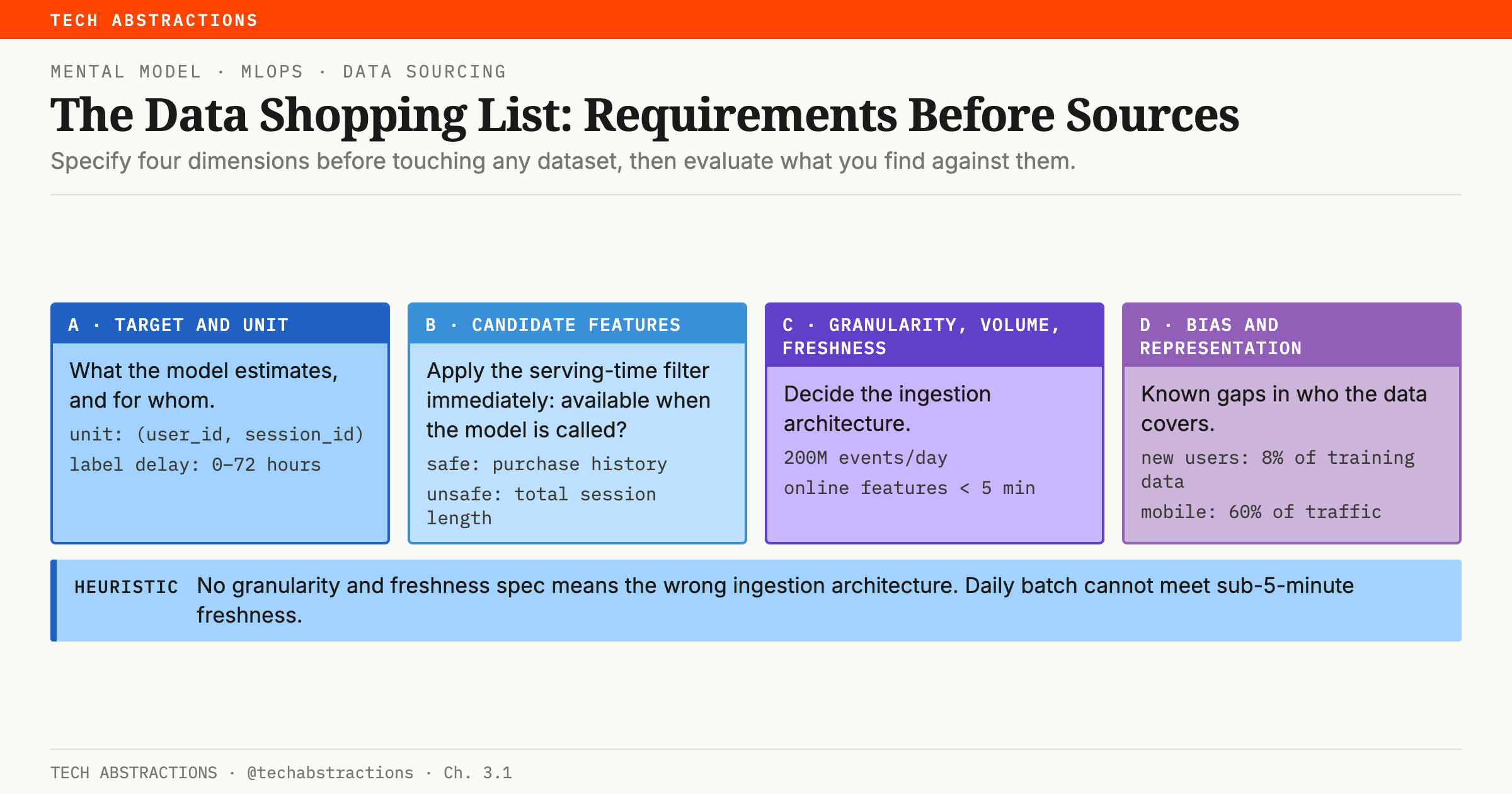
Before touching any dataset, a production ML team specifies four dimensions.
A. Target and unit of prediction
Every requirement flows from what the model is estimating and for whom. The unit of prediction determines the granularity of every feature and label in the system.
ShopSense, the running example in this course, is an e-commerce app with a product recommendation engine. Its target definition looks like this:
For ShopSense recommendation engine:
  Unit:          (user_id, session_id) pair
  Prediction:    Ordered list of product_ids to show
  Time horizon:  Next 10 minutes of session behavior
  Label:         Did the user click / add to cart / purchase?
  Label delay:   0–72 hours (purchase may complete later)
B. Candidate features: with serving-time filter applied immediately
List every signal that might predict the target. Then immediately apply the serving-time filter: which of these signals will be available when the model is called in production?
Available at serving time (safe):
  - user_id → historical purchase history (from the feature store, a service that serves precomputed features)
  - session events so far (from real-time event stream)
  - product metadata: category, price, inventory status

NOT available at serving time (dangerous if used):
  - "total session length" (not known until session ends)
  - "whether this product sold out in the next hour" (future information)
C. Granularity, volume, and freshness
Three properties that determine the ingestion architecture before a line of pipeline code is written.
Granularity: event-level user interactions (not aggregated sessions)
Volume:      200M events/day (10M daily active users × 20 events/session)
Freshness:   Training data: daily | Online features: < 5 minutes
If you cannot specify these three properties, you cannot choose an ingestion architecture. Daily batch is architecturally incompatible with sub-5-minute freshness requirements.
D. Bias and representation risks
ShopSense known gaps:
  - New users (<30 days): 8% of training data; model will perform
    poorly for 40% of users at any given time
  - Mobile-only users: different click patterns; desktop-trained
    model will underperform on mobile (60% of traffic)
The heuristic that prevents architecture mismatches: If you cannot specify granularity + freshness before choosing data sources, you will build the wrong ingestion architecture.
Think About It: The ShopSense Data Requirements
You're the ML lead at ShopSense and you're starting work on a new feature: a "Frequently Bought Together" section that appears on product detail pages. The product manager wants it live in 6 weeks.
Before looking at any data, work through the four requirements dimensions:
-
Unit of prediction: What is the entity this model predicts for? What does the model output? Is this a user-level model, a session-level model, or a product-pair model?
-
Serving-time filter: List 5 signals that intuitively seem useful for this feature. For each one, write: "Will this signal be available at the moment the product detail page loads?" Which signals are safe to use?
-
Freshness: The product manager says "the section should update daily." Is this the right freshness requirement? What would happen if a product sold out this morning but the "bought together" recommendation still showed it? What freshness would you argue for?
-
Representation bias: ShopSense has 50M SKUs but 80% of purchases are concentrated in 200K products. What does this imply about training data coverage for the long tail? What's the risk for the product if you ignore this?
There's no single right answer. The goal is to surface the constraints before touching data.
Source taxonomy: what every source type is good for
Once requirements are written, evaluate candidate sources against them. Every source type has a distinct failure mode. Matching source characteristics to requirements prevents the majority of production data failures.
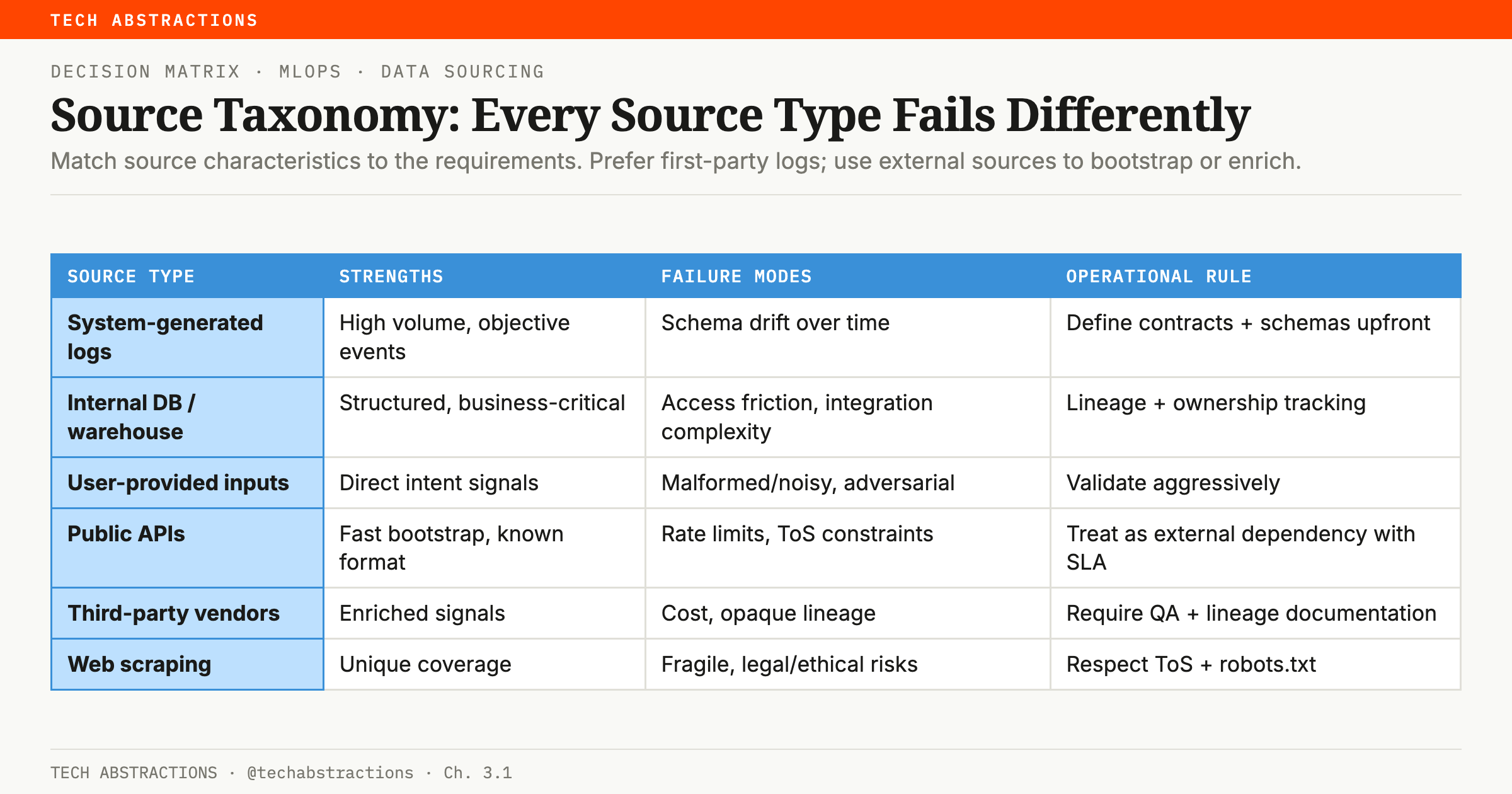
| Source type | Strengths | Failure modes | Operational rule |
|---|---|---|---|
| System-generated logs | High volume, objective events | Schema drift over time | Define contracts + schemas upfront |
| Internal DB / warehouse | Structured, business-critical | Access friction, integration complexity | Lineage + ownership tracking required |
| User-provided inputs | Direct intent signals | Malformed/noisy, adversarial | Validate aggressively |
| Public APIs | Fast bootstrap, known format | Rate limits, ToS constraints | Treat as external dependency with SLA |
| Third-party vendors | Enriched signals | Cost, opaque lineage | Require QA + lineage documentation |
| Web scraping | Unique coverage | Fragile, legal/ethical risks | Respect ToS + robots.txt |
The first-party preference rule: Prefer first-party system logs for long-term production value. Use external sources for bootstrapping or enrichment only.
First-party logs give you three properties that external sources cannot: ownership (you control the schema), freshness (you set the SLA), and lineage (you know where every field came from). When an external API changes its schema, your pipeline breaks silently. When a third-party vendor stops providing a feature, you discover it in production metrics.
Training-serving skew: a leading source of production bugs
Training-serving skew is the condition where a feature is computed differently at training time than at serving time. The model learns patterns from one distribution and is called with inputs from another. It is one of the most common root causes of production ML failures that look like model quality problems but are actually data pipeline problems.
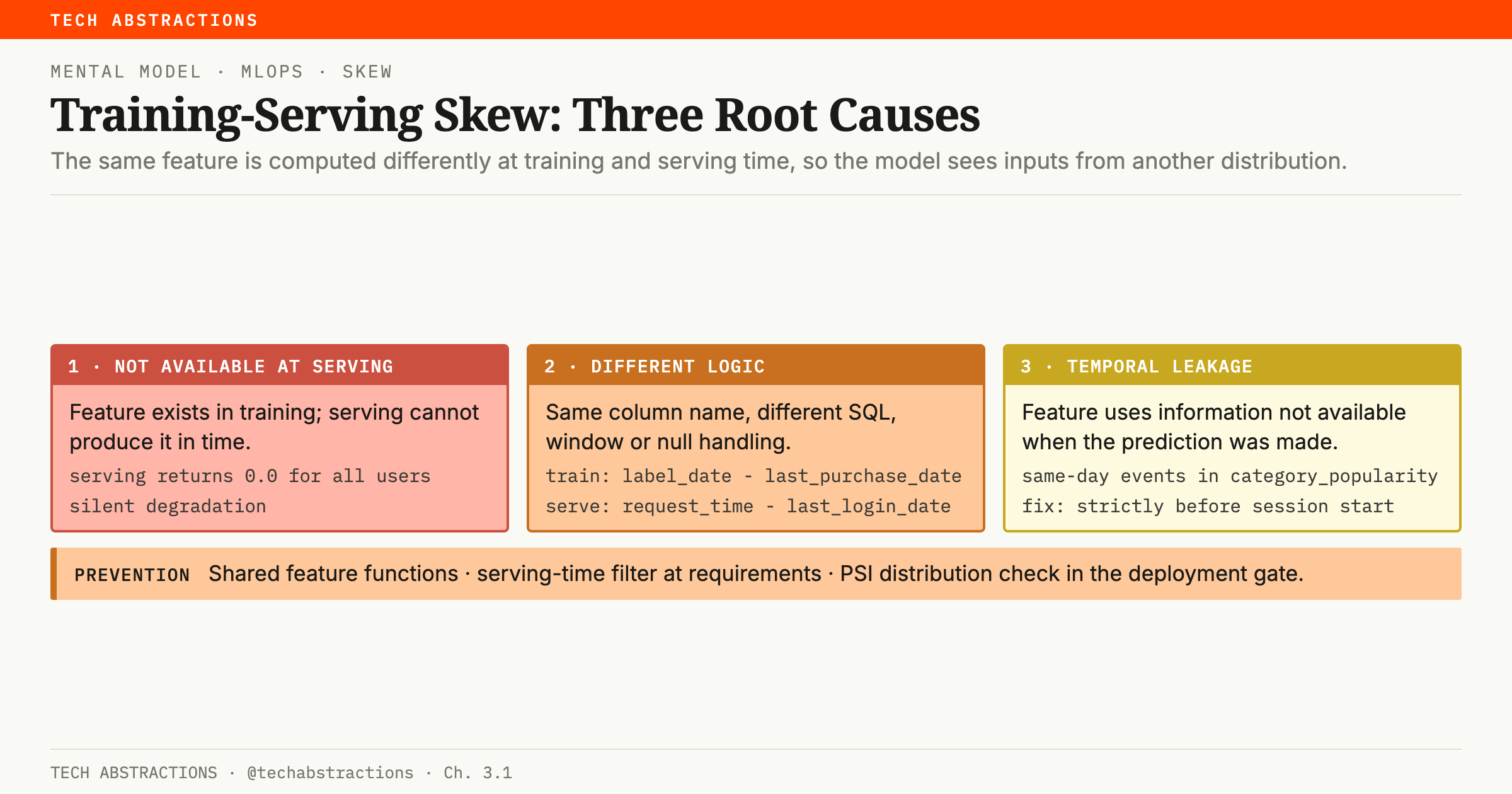
Root cause 1: Feature not available at serving time
The feature exists in the training dataset but the serving pipeline doesn't produce it or can't produce it in time.
# Training: computes user_avg_purchase_value_30d from warehouse (overnight batch)
# Serving: this feature was "forgotten" — serving API returns 0.0 for all users
# Model was trained on real values, deployed with all-zero values → silent degradation
Root cause 2: Feature computed with different logic
The same logical feature computed with different SQL, different windows, or different null handling.
# Training: recency = (label_date - last_purchase_date).days
# Serving:  recency = (request_time - last_login_date).days
# Same column name. Different meaning. Model degrades for regular purchasers.
Root cause 3: Temporal leakage
A feature computed using information that wasn't available at the time the prediction would have been made.
# WRONG: category_popularity includes events from same day as label
SELECT COUNT(*) AS category_popularity     -- ← leaks future info
FROM product_events p
WHERE DATE(p.event_time) = DATE(u.session_date)  -- ← same day!

# CORRECT: only events strictly before session start
WHERE DATE(p.event_time) < DATE(u.session_date)  -- ← strict before
Prevention protocol: three rules that prevent training-serving skew:
- Shared feature functions: The same Python function that computes a feature in training must be called from serving. Two codepaths will diverge.
- Serving-time filter at requirements phase: For every candidate feature: "Will this exact signal be available at the moment of the serving request?"
- PSI distribution check in deployment gate: Compare each feature's training distribution with a live serving sample using the population stability index (PSI), a score of how far one distribution has drifted from another. A common rule of thumb treats PSI above 0.2 as a significant shift; if any feature crosses it, block deployment.
Think About It: Diagnosing a Training-Serving Skew
Your recommendation engine has been in production for 3 months. Offline evaluation shows Recall@10 = 0.095. You deploy and observe click-through rate drop from the expected 2.8% to 1.4% in the first week, a 50% gap between offline and online performance.
You're asked to diagnose whether this is a model quality issue or a data pipeline issue.
- What's the first check you'd run, and what tool would you use?
- You pull a sample of 1,000 real serving requests and compare the feature values to the training set. You observe that
user_purchase_count_30dhas mean=4.2 in training but mean=0.3 in serving. What does this tell you? List at least 2 hypotheses for what went wrong. - You check the feature store and discover that
user_purchase_count_30dis computed correctly in the online store, but only for users who made at least one purchase in the last 90 days. New users and churned users return 0.0. Your training dataset included all users but weighted toward active purchasers. What is the exact mechanism of skew here? - The fix is to either (a) retrain with a training dataset filtered to only users with valid purchase history, or (b) update the serving pipeline to handle cold-start users explicitly. Which do you pick and why?
Storage decisions: land raw first, curate second
The default storage architecture for ML data is the two-zone pattern: raw zone and curated zone.
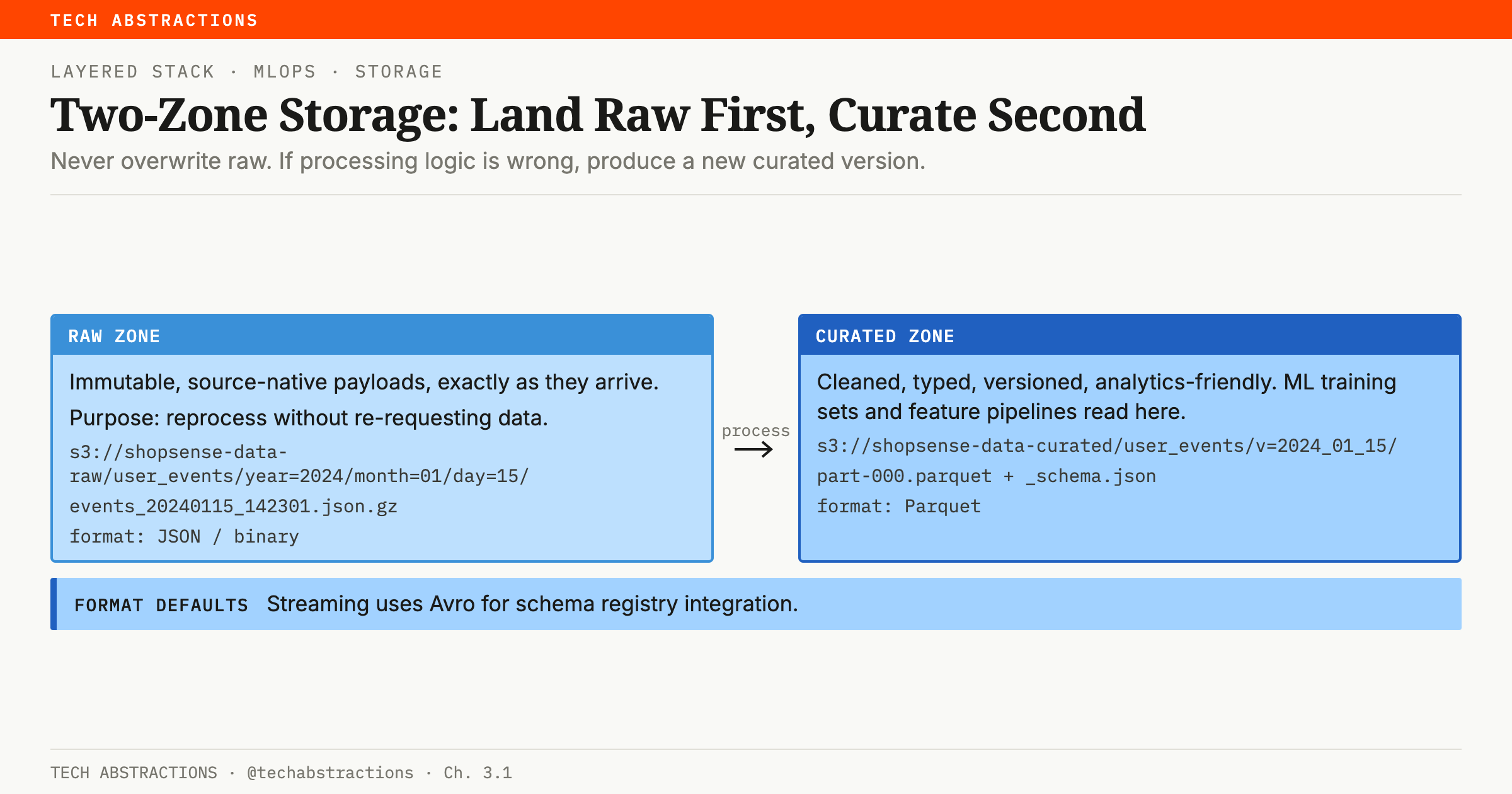
Raw zone: immutable, source-native payloads
Stores data exactly as it arrives from the source, before any transformation. Nothing in the raw zone is ever overwritten. The purpose is reprocessability: if you discover a processing bug three months after ingestion, you reprocess from raw without re-requesting data.
Curated zone: cleaned, typed, versioned, analytics-friendly
Parquet tables with explicit schema versions. This is where ML training datasets live and feature pipelines read from.
Raw zone:    s3://shopsense-data-raw/user_events/year=2024/month=01/day=15/
             → events_20240115_142301.json.gz (source-native, immutable)

Curated:     s3://shopsense-data-curated/user_events/v=2024_01_15/
             → part-000.parquet + _schema.json (versioned, typed)
Rule: Never overwrite raw. If processing logic is wrong, produce a new curated version.
Format defaults: Curated → Parquet (columnar, compressed, schema evolution). Raw → JSON/binary (source-native). Streaming → Avro (schema registry integration).
Data versioning: non-negotiable for reproducibility
You need to be able to answer: "Which exact data produced this model?" Without this, you cannot reproduce training results, debug model regressions, or satisfy audit requirements.
Minimum viable data versioning requires four things:
1. Dataset snapshot IDs: every training dataset has a unique, deterministic ID
def compute_dataset_version(data_paths: list[str]) -> str:
    hasher = hashlib.sha256()
    for path in sorted(data_paths):
        hasher.update(path.encode())
        with Path(path).open("rb") as f:  # hash contents, not mtime
            for chunk in iter(lambda: f.read(1 << 20), b""):
                hasher.update(chunk)
    return hasher.hexdigest()[:16]
2. A version manifest: ties together the artifacts needed for reproducibility:
version: "20240115_a3b8c2d1"
artifacts:
  code_commit: "abc123def456"
  training_data_path: "s3://shopsense-data-curated/user_events/v=2024_01_15/"
  feature_schema_version: "user_features_v3.2"
  environment_digest: "sha256:e3b0c44298fc..."
3. Immutable dataset paths: once linked to a model, a curated dataset version must not be modified.
4. Model artifact → dataset linkage: the model in the registry must reference the dataset version it was trained on.
EDA as a production activity: not a notebook ritual
Exploratory Data Analysis in production ML has a different purpose than academic EDA. The goal is not to produce visualizations. The goal is to make decisions: is this dataset suitable? What preprocessing is required? What are the failure modes that need monitoring?
EDA output should become tests. The distribution you observe becomes the schema contract that runs in CI. The null rate you measure becomes the threshold in the data quality check.
The minimum EDA checklist
Every dataset used in ML training must pass through this checklist before any feature engineering:
□ Schema and types — consistent with what serving will produce?
□ Missing values per field — which fields have nulls? Are nulls random or systematic?
□ Distributions and long tails — require clipping or log transforms?
□ Label balance and slice balance — stable across time, cohorts, categories?
□ Duplicates and entity collisions — duplicate events, account merges?
□ Time-based leakage checks — feature timestamp always before label timestamp?
□ Sample record sanity review — read 20–50 records manually
The discipline: Convert EDA findings into executable checks.
# EDA finding: user_purchase_count has 0.3% null rate, max value 4,821

class TestUserPurchaseCountContract:
    def test_null_rate_within_threshold(self, user_features: pd.DataFrame):
        null_rate = user_features["user_purchase_count"].isna().mean()
        assert null_rate < 0.01, f"Null rate {null_rate:.3%} exceeds 1% threshold"

    def test_no_extreme_outliers(self, user_features: pd.DataFrame):
        p999 = user_features["user_purchase_count"].quantile(0.999)
        assert p999 < 2000, f"P99.9 value {p999} suggests data quality issue"
Think About It: EDA Finding, Cold-Start Sparsity
You run the minimum EDA checklist on ShopSense's user interaction data and find:
user_purchase_count_lifetime:
  mean = 8.3
  median = 2.0
  p90 = 18.0
  p99 = 124.0
  null_rate = 0.0%
  value_counts:
    0-1 purchases: 42% of users
    2-10 purchases: 38% of users
    11+ purchases: 20% of users
-
What does this distribution tell you about the cold-start problem for a collaborative filtering recommendation model? Specifically: if you train on this data, which users will the model perform worst on?
-
The label in your training dataset is
clicked_recommended_product(binary). The click rate across all users is 2.1%. You compute the click rate by cohort:- 0-1 purchases: 0.4% click rate
- 2-10 purchases: 2.8% click rate
- 11+ purchases: 6.2% click rate
What does this mean for model evaluation? If you report "Recall@10 = 0.09" as your offline metric, what is it hiding?
-
What EDA finding would you convert into a production monitoring check? Write the check as pseudocode or a test assertion.
Data documentation: preventing data folklore
At a small team, knowledge of which datasets are trustworthy lives in Slack threads and senior engineers' memories. This is data folklore, and it does not scale.
Data folklore creates five failure modes: engineers reuse datasets for tasks they weren't designed for; models get retrained on data whose known issues were forgotten; new team members spend weeks rediscovering what senior engineers already know; postmortems cannot determine which data trained which model; regulatory audits require lineage that doesn't exist.
The solution is structured data documentation: a machine-readable data card that captures dataset properties in a standard format that can be versioned, queried, and linked to models.
Minimal data card template
name: "user_events"
version: "3.2"
owner: "data-platform-team"
source:
  system: "Kafka → S3 event pipeline"
  ingestion_method: "streaming → batch consolidation (hourly)"
freshness:
  update_frequency: "hourly"
  sla_hours: 2
quality:
  known_issues:
    - "0.3% null rate on product_id for search events"
    - "Duplicate events possible for mobile clients — deduplicate with 5-min window"
governance:
  pii_fields: ["user_id (hashed)", "ip_address (NOT present — stripped at ingestion)"]
  retention_days: 548
  usage_restrictions: "ML training and analytics only"
lineage:
  downstream_models: ["recommendation-engine-v*", "demand-forecasting-v*"]
  downstream_features: "feast://feature-store/user_behavior_features"
When to adopt a data catalog platform: Start with YAML data cards + a versioned manifest. Adopt a catalog (DataHub, Amundsen, OpenMetadata) when repeated "where is this data?" cycles across teams, column-level lineage, or governance enforcement requirements make the manual approach a bottleneck.
Early governance: do it before the incident
Data governance decisions made early are architectural. Decisions made after a compliance incident are emergency surgery.
Three governance actions at data sourcing time:
1. PII identification
Walk through every field. For each field: does this contain or could it be combined with other fields to produce information that identifies a natural person?
ShopSense user events:
  user_id:     Pseudonymous (hashed): not raw PII, but still personal data under GDPR
  ip_address:  Raw IP → strip at ingestion, do not store
  device_id:   Could identify device → classify as PII
  location:    City-level OK; GPS coordinates → PII
2. Access control via least privilege
Define IAM roles per pipeline stage before any pipeline is built.
data_ingestion_pipeline:
  read:  [app event kafka topic]
  write: [s3://shopsense-data-raw/]

feature_engineering_pipeline:
  read:  [s3://shopsense-data-curated/]
  write: [feast://offline-store/]

ml_training_pipeline:
  read:  [feast://offline-store/]
  write: [mlflow://experiments/]
3. Terms of Service compliance
Any external data source is a dependency with legal failure modes. Document where the ToS is located, confirm ML training is permitted, record the date of review.
Operational deliverables: what "done" looks like
Data sourcing is complete when you can check all seven items:
✅ Data requirements document
   - Unit of prediction, candidate features with serving-time filter,
     granularity + volume + freshness, bias risks

✅ Source inventory
   - Every source: location, owner, access method, SLA, ToS review

✅ Two-zone storage layout
   - Raw zone paths (immutable), curated zone paths (versioned)

✅ Dataset versioning approach
   - Snapshot ID convention, version manifest format, model artifact ↔ dataset link

✅ EDA notebook + written findings summary
   - Minimum checklist complete, findings converted to test specifications

✅ Data cards for all primary datasets
   - Owner, schema, freshness SLA, known issues, lineage (YAML)

✅ Governance groundwork
   - PII fields identified, access roles defined, ToS compliance documented
Case Study: Instacart's Recommendation Degradation (2021)
Instacart's ML team described a recommendation quality incident where performance degraded significantly in production despite strong offline metrics. The root cause was training-serving skew introduced during a data pipeline migration.
What happened: The team migrated user behavior data from batch ETL to streaming. The batch pipeline computed user purchase frequency over a rolling 7-day window using midnight-to-midnight UTC timestamps. The new streaming pipeline computed the same feature using a trailing 168-hour window from current request time.
Both compute "7-day purchase frequency." Both implementations look equivalent. In practice they produce different values for every request. The batch version aligns with natural user behavior patterns (weekend shopping, weekly grocery runs); the streaming version's window shifts continuously.
The model had learned the batch-computed distribution. In production it received streaming-computed values. For users with regular weekly patterns, a major Instacart cohort, the distributions diverged significantly. Click-through rate dropped 12% before the cause was identified.
Fix: Introduced a shared feature definition library imported by both pipelines. Feature logic was written once, with timestamp convention made explicit. A PSI-based offline/online distribution check was added to the deployment gate.
What would you change?
The team detected the skew via click-through rate drop, a business metric. This took days. Three earlier detection points existed that would have caught this before it reached production:
- A training/serving distribution comparison run during model deployment validation, comparing feature distributions between the training set and a live serving sample
- A feature definition review during the pipeline migration code review, a checklist item: "Does this migration change any feature computation semantics?"
- A canary deployment PSI check: monitoring feature PSI in the 5% canary traffic before full rollout
Question for reflection: The team chose to fix the problem by creating a shared feature library. An alternative would have been to retrain the model on data produced by the new streaming pipeline (accepting the new semantics). What are the trade-offs between these two approaches? Which would you choose and why?
Expert analysis:
The shared feature library approach (what Instacart chose) is almost always correct because:
- It preserves the semantics the model learned during training
- It fixes the root cause (dual implementations) rather than the symptom (distribution mismatch)
- Retraining on the streaming semantics takes weeks; the shared library fix can be deployed in hours
- Future feature additions will automatically use the same library, preventing recurrence
Retraining on streaming semantics makes sense only if: (1) the streaming semantics are intentionally better than the batch semantics (not the case here), or (2) the cost of maintaining dual compute paths is higher than the retraining cost (rare).
Lesson: "Same feature name, different implementation" is harder to detect than "feature missing entirely." Add training vs. serving distribution comparison (PSI check per feature) to your model deployment checklist.
Case Study: Netflix's Data Contract Program (2022)
Netflix engineering tackled the problem of data trust at scale. The core insight: metadata freshness was harder than metadata richness. They had a catalog. The catalog wasn't trusted.
Context: Netflix's data catalog had been built over several years. By 2021, data practitioners reported that they couldn't trust catalog entries: ownership information was stale after org changes, schema descriptions were outdated after pipeline migrations, "known issues" sections were empty for datasets with real known problems. The catalog existed but wasn't used.
The four design decisions Netflix made:
Decision 1: Push-based metadata over crawl-based
Old approach: catalog crawlers ran nightly and pulled schema/stats from each dataset location. New approach: pipeline jobs were required to emit metadata events on every successful run: schema validation results, record counts, SLA compliance, null rates for key fields.
Why this mattered: A crawl-based system is always one step behind. If a pipeline runs at 2am and the crawler runs at 3am, metadata is already 1 hour old by the time it's indexed. More critically, if the pipeline fails, the crawler has nothing new to ingest, but the catalog shows the last successful run as "current." Push-based metadata is emitted by the pipeline itself, so failure is visible immediately.
Decision 2: Separate operational metadata (automated) from interpretive metadata (human)
Old approach: a single metadata form that engineers filled in manually. New approach: operational metadata (freshness, schema, volume, quality metrics) is 100% automated via pipeline emissions. Interpretive metadata (description, known issues, business context, usage restrictions) is human-authored, with lightweight tooling to make it easy.
Why this mattered: Engineers were failing to maintain operational metadata because it's tedious and error-prone to manually update "last_updated: 2024-01-15" when you can just emit it automatically. Separating the two concerns means operational metadata is always accurate, and humans focus on the parts they're actually good at: judgment and context.
Decision 3: Data contracts as deployment gates
Any dataset consumed by a production ML model required a machine-readable data contract: schema specification, freshness SLA, and minimum quality thresholds. Training pipelines that attempted to read from datasets without a valid, non-expired contract would fail at the pipeline integration step.
Why this mattered: It created a forcing function. Teams couldn't skip documentation as a "we'll do it later" item. The contract had to exist before training could proceed. This also meant that when a dataset's schema changed, the contract had to be updated, which triggered a notification to downstream consumers.
Decision 4: Contract versioning, not dataset versioning alone
The data contract itself was versioned (not just the dataset). When a contract was updated (schema addition, freshness SLA change), the version bumped. Downstream models tracked which contract version they were validated against.
Why this mattered: It created an audit trail. For any production model, you could answer: "What did the team know about this dataset at the time this model was trained?", including known issues, quality thresholds, and schema expectations.
Questions for analysis:
-
Decision 3 creates a forcing function but also creates friction. A new team starting a project can't train their first model until they've written data contracts. How would you balance enforcement strictness against onboarding friction for new teams?
-
Netflix enforces data contracts at "pipeline integration time", meaning the training pipeline fails if it tries to read a contract-less dataset. An alternative is to enforce at "model deployment time": the training runs, but the model can't be promoted to production without valid contracts. Which enforcement point is better? What does each approach miss?
-
The push-based metadata approach requires that all data pipelines emit metadata events. What happens to datasets that are produced by legacy pipelines that haven't been updated to emit metadata? How would you handle this migration in practice?
-
Data contracts encode the team's knowledge about a dataset at a point in time. A contract written in January may be incorrect by March if upstream data changes. How would Netflix's system detect contract drift, the case where the contract still says "null_rate < 0.5%" but the actual null rate is now 12%?
Advanced Exercise 1: Write a Data Requirements Document
Scenario: ShopSense is building a second ML system: a demand forecasting model that predicts weekly product-level demand 4 weeks ahead, used by the inventory team to set reorder quantities. You've been asked to write the Data Requirements Document before any data sourcing begins.
The business context:
- 50M SKUs across 40 product categories
- Inventory decisions made weekly (Monday planning cycle)
- Current process: manual analyst forecasting for top 10K SKUs, rule-based for the rest
- ML goal: improve forecast accuracy (WMAPE) by ≥ 20% vs. current process for the top 100K SKUs
- Risk: over-forecasting leads to excess inventory cost; under-forecasting leads to stockouts (lost revenue)
Task: Write a complete Data Requirements Document with all seven required sections:
## Data Requirements Document: ShopSense Demand Forecasting

### 1. Unit of Prediction
[Define: What is the entity? What is the prediction output? What is the time horizon?]

### 2. Candidate Features with Serving-Time Filter
[List at least 8 candidate signals. For each: is it available at prediction time?
Mark each: ✓ Safe | ✗ Exclude | ⚠ Available but with lag]

### 3. Granularity, Volume, and Freshness Requirements
[Specify each of the three properties explicitly. Explain which ingestion
architecture is implied by the freshness requirement.]

### 4. Label Definition and Label Delay
[What is the label? When does it arrive after prediction time?
What does this imply for the training pipeline's label join?]

### 5. Bias and Representation Risks
[Identify at least 3 systematic gaps in the training data.
For each: what population is under-represented, and what's the model consequence?]

### 6. Candidate Source Inventory
[For each data signal identified, specify: source system, freshness, tier (1/2/3),
known failure mode]

### 7. Data Sourcing Acceptance Criteria
[7 checkbox criteria that must be true before the data sourcing phase is "done"]
Acceptance criteria for your document:
- Unit of prediction specifies entity, output format, and time horizon
- Serving-time filter applied and documented for every feature candidate
- Freshness requirement translates to a specific ingestion architecture choice
- Label delay is quantified (not just "there is a label delay")
- At least 3 representation gaps identified with model consequence named
- Every source in the inventory has a tier assignment and failure mode
Advanced Exercise 2: Training-Serving Skew Detection
Scenario: A ShopSense data engineer has submitted a pull request that introduces a new feature for the recommendation model: item_view_velocity_1h, the number of times a product was viewed in the last hour across all users. The PR adds this feature to the training pipeline. You are reviewing it.
The PR includes this training-side feature computation:
def compute_item_view_velocity_1h(
    product_id: str,
    label_timestamp: datetime,
    events_df: pd.DataFrame,
) -> int:
    """Count views of this product in the hour before label_timestamp."""
    window_start = label_timestamp - timedelta(hours=1)
    return len(events_df[
        (events_df["product_id"] == product_id) &
        (events_df["event_type"] == "view") &
        (events_df["event_time"] >= window_start) &
        (events_df["event_time"] < label_timestamp)
    ])
The serving pipeline reads this feature from the feature store:
# In the online feature store (Redis), this feature is populated by:
# A Kafka consumer that counts views per product with a 1-hour tumbling window
# Window resets at :00 of each hour (00:00, 01:00, 02:00, ...)

def get_online_item_view_velocity(product_id: str) -> int:
    redis_key = f"item_velocity:{product_id}:current_hour"
    return int(redis_client.get(redis_key) or 0)
Questions:
-
Identify the skew: There is a training-serving skew in this feature. Describe it precisely. When is the skew largest? When is it smallest?
-
Quantify the impact: At 12:59pm,
product_id="SHOES_123"has had 45 views since 12:00pm. The training-side code would compute velocity=45. The serving-side code would compute velocity=45. At 1:00pm exactly, the window resets. What does the training side return for a prediction made at 1:01pm for a product with 5 views in the last minute? What does the serving side return? -
Design the fix: Write a corrected version of the serving-side feature computation that eliminates the semantic gap. You can choose either: (a) fix the serving side to match the training semantics, or (b) fix the training side to match the serving semantics. State which you chose and why.
-
Write the contract test: The PR should include a test that validates the training and serving feature implementations produce the same output for a given input. Write this test.
class TestItemViewVelocityContract:
    """
    Contract: training-side and serving-side implementations of
    item_view_velocity_1h must produce identical outputs for the same
    product, timestamp, and event history.
    """
    def test_implementations_agree_mid_hour(self, events_df, redis_client):
        # Your test here
        pass

    def test_implementations_agree_at_hour_boundary(self, events_df, redis_client):
        # This is the edge case where the skew manifests
        pass
Advanced Exercise 3: EDA Decision Tree for Production
Scenario: You've been given a dataset of ShopSense user sessions for training the recommendation model. The dataset covers roughly 11 weeks (Oct 1 to Dec 15) and contains 180M sessions. Run through the minimum EDA checklist and answer each decision question.
Dataset statistics you've computed:
user_id:                    180M rows, 0% null, 8.2M unique users
session_id:                 180M rows, 0% null, 180M unique (good)
session_start_time:         180M rows, 0% null, range: 2023-10-01 to 2023-12-15
session_duration_seconds:   180M rows, 2.1% null, mean=487, median=180, p99=8,400
                            max=86,400 (= 24 hours — suspicious)
event_count:                180M rows, 0% null, mean=18.3, median=11, p99=142, max=4,821
purchased:                  180M rows, 0% null, mean=0.021 (2.1% positive rate)
first_product_category:     180M rows, 3.8% null, 847 unique values
user_purchase_count_lifetime: 180M rows, 0.0% null, mean=8.3, median=2, p99=124, max=9,847

Temporal distribution:
  October: 62M sessions
  November: 71M sessions
  December: 47M sessions (truncated — data through Dec 15 only)
Work through the checklist:
-
Schema check: You notice
session_duration_secondshas a max of 86,400 (24 hours). Three possible explanations: (a) bot/crawler sessions, (b) users who left a tab open, (c) a data pipeline bug. How do you determine which? What would each distribution look like in a histogram? -
Label balance check: The positive rate is 2.1% overall. You compute it by month:
- October: 2.3%
- November: 2.8%
- December: 1.4%
The December rate is 50% lower. Is this a data quality issue or a real business effect? How do you determine which? What does the answer imply for your train/validation/test split?
-
Temporal leakage check: Your label is
purchased(did the user purchase anything in this session). Your training feature includesuser_purchase_count_lifetime(total lifetime purchases). Explain why this feature is valid (not leakage) even though it's correlated with the label. Now explain a modification of this feature that would constitute leakage. -
Sparsity decision: 42% of users have ≤ 1 lifetime purchase. For a collaborative filtering model, these users have essentially no purchase history signal. You have three options:
- (a) Include them in training (cold-start problem, model performance is poor for this group)
- (b) Exclude them from training (train on warm users only)
- (c) Train separate models (one for cold-start, one for warm users)
What are the trade-offs? What additional information would you need to make this decision?
-
EDA → Tests: Convert your finding about
session_duration_secondsmax value into a data quality test specification. Include: test name, input, expected behavior, and what action should be triggered on failure.
Real-World Implementation 1: DVC Data Versioning for ShopSense
Objective: Set up DVC (Data Version Control) data versioning for the ShopSense recommendation engine training dataset. Track dataset snapshots so that every model training run can be reproduced from the exact data it used.
Part A: DVC setup
# 1. Initialize DVC in the project repo
cd shopsense-ml-repo
dvc init

# 2. Configure remote storage (S3)
dvc remote add -d s3remote s3://shopsense-dvc-storage/recommendation/
dvc remote modify s3remote region us-east-1

# 3. Create the dataset directory structure
mkdir -p data/raw data/curated data/training

# Note: `dvc add` automatically adds the data it tracks to .gitignore, so git
# stores only the small .dvc pointer files. (.dvcignore is a different file:
# it tells DVC which files to skip when it scans a directory.)
Part B: Versioning a training snapshot
# scripts/create_training_snapshot.py

import subprocess
import hashlib
import json
import yaml
from datetime import datetime, timezone
from pathlib import Path
from typing import Any


def compute_content_hash(file_paths: list[Path]) -> str:
    """Compute SHA256 hash of file contents (not metadata) for reproducibility."""
    hasher = hashlib.sha256()
    for path in sorted(file_paths):
        if path.exists():
            hasher.update(path.read_bytes())
    return hasher.hexdigest()[:16]


def create_training_snapshot(
    curated_data_dir: Path,
    output_dir: Path,
    training_config: dict[str, Any],
) -> dict[str, Any]:
    """
    Create a versioned training snapshot from curated data.
    Returns the version manifest that must be logged to MLflow.
    """
    timestamp = datetime.now(timezone.utc).strftime("%Y%m%d_%H%M%S")

    # Collect all parquet files to include in this snapshot
    data_files = sorted(curated_data_dir.glob("**/*.parquet"))
    if not data_files:
        raise ValueError(f"No parquet files found in {curated_data_dir}")

    content_hash = compute_content_hash(data_files)
    version_id = f"{timestamp}_{content_hash}"

    # Create snapshot directory with versioned name
    snapshot_dir = output_dir / f"v={timestamp}"
    snapshot_dir.mkdir(parents=True, exist_ok=True)

    # Copy (or symlink) data files into snapshot
    for src in data_files:
        dst = snapshot_dir / src.name
        dst.write_bytes(src.read_bytes())

    # Get git commit of current code
    git_result = subprocess.run(
        ["git", "rev-parse", "HEAD"],
        capture_output=True,
        text=True,
        check=True,
    )
    code_commit = git_result.stdout.strip()

    # Write version manifest
    manifest = {
        "version": version_id,
        "created_at": datetime.now(timezone.utc).isoformat(),
        "artifacts": {
            "code_commit": code_commit,
            "training_data_path": str(snapshot_dir),
            "dvc_file": str(snapshot_dir) + ".dvc",
            "file_count": len(data_files),
            "content_hash": content_hash,
            "training_config": training_config,
        },
        "reproduction": {
            "restore_command": f"dvc checkout {snapshot_dir}.dvc",
            "notes": "Run 'dvc pull' before restoring if not already cached locally",
        },
    }

    manifest_path = snapshot_dir / "_version_manifest.yaml"
    with open(manifest_path, "w") as f:
        yaml.dump(manifest, f, default_flow_style=False, sort_keys=True)

    # Track with DVC only after the manifest is written, so the manifest is
    # part of the tracked snapshot (writing into a tracked directory afterwards
    # would make it differ from what DVC recorded).
    subprocess.run(["dvc", "add", str(snapshot_dir)], check=True, capture_output=True)
    subprocess.run(["dvc", "push"], check=True, capture_output=True)

    return manifest


if __name__ == "__main__":
    manifest = create_training_snapshot(
        curated_data_dir=Path("data/curated/user_events"),
        output_dir=Path("data/training"),
        training_config={
            "window_days": 90,
            "min_user_events": 2,
            "label": "purchased",
        },
    )
    print(f"Created training snapshot: {manifest['version']}")
    print(f"Manifest written to: data/training/v={manifest['version'][:15]}/_version_manifest.yaml")
Part C: Logging version to MLflow
import mlflow
import yaml
from pathlib import Path


def train_with_versioning(snapshot_dir: Path, model_config: dict):
    """Training run that logs dataset version for full reproducibility."""
    manifest_path = snapshot_dir / "_version_manifest.yaml"
    with open(manifest_path) as f:
        manifest = yaml.safe_load(f)

    with mlflow.start_run() as run:
        # Log dataset version as a parameter (enables filtering by dataset in UI)
        mlflow.log_param("dataset_version", manifest["version"])
        mlflow.log_param("dataset_content_hash", manifest["artifacts"]["content_hash"])
        mlflow.log_param("training_data_path", manifest["artifacts"]["training_data_path"])
        mlflow.log_param("code_commit", manifest["artifacts"]["code_commit"])

        # Log the full manifest as an artifact for complete reproducibility
        mlflow.log_artifact(str(manifest_path), "dataset_metadata")

        # ... training code here ...

        return run.info.run_id
Part D: Verification exercise
After running the setup above:
-
Make a small change to one data file in
data/curated/. Runcreate_training_snapshot()again. Verify that the new snapshot has a differentversionID. Why does the content hash change? -
Delete the local
data/training/directory. Rundvc checkoutto restore the snapshot from S3 remote. Does the restored data match the original? How do you verify this? -
In a CI pipeline that runs model training, where should
dvc pullbe called, before the training step or as part of the training step itself? What breaks if you forget to calldvc pull?
Real-World Implementation 2: Data Card Generator
Objective: Write a Python script that reads a Parquet dataset and automatically generates a structured YAML data card. The generated card covers all required fields; human-authored fields (description, known issues, usage restrictions) are left as prompts.
# scripts/generate_data_card.py
"""
Generates a data card YAML from a Parquet dataset.
Automated fields are populated from the data; human fields are left as prompts.
"""

import hashlib
import json
from datetime import datetime, timezone
from pathlib import Path
from typing import Any

import pandas as pd
import pyarrow.parquet as pq
import yaml


def compute_field_stats(df: pd.DataFrame, col: str) -> dict[str, Any]:
    """Compute schema + quality statistics for a single column."""
    series = df[col]
    stats: dict[str, Any] = {
        "name": col,
        "dtype": str(series.dtype),
        "null_rate": round(float(series.isna().mean()), 6),
        "unique_count": int(series.nunique()),
        "row_count": len(series),
    }

    if pd.api.types.is_bool_dtype(series):
        # bool is "numeric" to pandas, but quantile() fails on it
        stats["bool_stats"] = {"true_rate": round(float(series.dropna().mean()), 4) if series.notna().any() else None}

    elif pd.api.types.is_numeric_dtype(series):
        non_null = series.dropna()
        if len(non_null) > 0:
            stats["numeric_stats"] = {
                "mean": round(float(non_null.mean()), 4),
                "std": round(float(non_null.std()), 4),
                "min": round(float(non_null.min()), 4),
                "p25": round(float(non_null.quantile(0.25)), 4),
                "median": round(float(non_null.median()), 4),
                "p75": round(float(non_null.quantile(0.75)), 4),
                "p95": round(float(non_null.quantile(0.95)), 4),
                "p99": round(float(non_null.quantile(0.99)), 4),
                "max": round(float(non_null.max()), 4),
            }

    elif pd.api.types.is_string_dtype(series) or pd.api.types.is_object_dtype(series):
        non_null = series.dropna().astype(str)
        if len(non_null) > 0:
            value_counts = non_null.value_counts()
            stats["string_stats"] = {
                "top_5_values": [
                    {"value": str(v), "count": int(c)}
                    for v, c in value_counts.head(5).items()
                ],
                "is_high_cardinality": bool(series.nunique() > 100),
            }

    elif pd.api.types.is_datetime64_any_dtype(series):
        non_null = series.dropna()
        if len(non_null) > 0:
            stats["temporal_stats"] = {
                "min": str(non_null.min()),
                "max": str(non_null.max()),
                "range_days": int((non_null.max() - non_null.min()).days),
            }

    return stats


def compute_dataset_hash(parquet_paths: list[Path]) -> str:
    """Compute content hash of Parquet files for versioning."""
    hasher = hashlib.sha256()
    for path in sorted(parquet_paths):
        hasher.update(path.read_bytes())
    return hasher.hexdigest()[:16]


def generate_data_card(
    parquet_dir: Path,
    dataset_name: str,
    owner: str,
    output_path: Path | None = None,
) -> dict[str, Any]:
    """
    Generate a data card YAML from a Parquet dataset directory.

    Human-authored fields are left with '<<REQUIRED: ...>>' prompts.
    Automated fields are populated from the data.
    """
    parquet_files = sorted(parquet_dir.glob("*.parquet"))
    if not parquet_files:
        raise FileNotFoundError(f"No .parquet files found in {parquet_dir}")

    # Read a sample for profiling (first 100K rows of each file)
    dfs = []
    total_rows = 0
    for pf in parquet_files:
        pq_file = pq.ParquetFile(pf)
        total_rows += pq_file.metadata.num_rows
        dfs.append(pd.read_parquet(pf).head(100_000))
    df = pd.concat(dfs, ignore_index=True)

    content_hash = compute_dataset_hash(parquet_files)

    # Build field-level statistics
    field_stats = [compute_field_stats(df, col) for col in df.columns]

    # Detect potential PII fields by name heuristics
    pii_heuristic_keywords = [
        "email", "phone", "name", "address", "ip", "ssn",
        "passport", "dob", "birth", "location", "geo", "lat", "lon",
        "device_id", "mac_address",
    ]
    potential_pii = [
        col for col in df.columns
        if any(kw in col.lower() for kw in pii_heuristic_keywords)
    ]

    card: dict[str, Any] = {
        "name": dataset_name,
        "version": f"auto_{content_hash}",
        "generated_at": datetime.now(timezone.utc).isoformat(),
        "generated_by": "generate_data_card.py (automated)",
        "owner": owner,

        # Human-authored fields — left as prompts
        "description": "<<REQUIRED: What is this dataset and what is it for?>>",
        "source": {
            "system": "<<REQUIRED: Which system/pipeline produces this data?>>",
            "ingestion_method": "<<REQUIRED: batch/streaming/snapshot?>>",
            "upstream_systems": "<<REQUIRED: List upstream data sources>>",
        },

        # Automated fields
        "schema": {
            "row_count_total": total_rows,
            "file_count": len(parquet_files),
            "content_hash": content_hash,
            "columns": field_stats,
        },

        "freshness": {
            "update_frequency": "<<REQUIRED: hourly/daily/weekly/on-demand?>>",
            "sla_hours": "<<REQUIRED: Maximum acceptable staleness in hours>>",
            "monitoring_alert": "<<REQUIRED: Where is SLA alerting configured?>>",
        },

        "quality": {
            "auto_detected_issues": _detect_quality_issues(df, field_stats),
            "known_issues": ["<<REQUIRED: List known data quality issues>>"],
            "quality_tests": "<<REQUIRED: Path to data quality test file>>",
        },

        "governance": {
            "potential_pii_fields": potential_pii if potential_pii else [],
            "pii_review_required": len(potential_pii) > 0,
            "confirmed_pii_fields": "<<REQUIRED: After PII review, list confirmed PII fields>>",
            "access_role": "<<REQUIRED: IAM role required for access>>",
            "retention_days": "<<REQUIRED: Retention period in days>>",
            "deletion_strategy": "<<REQUIRED: How are deletion requests handled?>>",
            "usage_restrictions": "<<REQUIRED: Permitted use cases>>",
        },

        "lineage": {
            "upstream_datasets": "<<REQUIRED: List upstream datasets this is derived from>>",
            "downstream_models": "<<REQUIRED: List models that use this dataset>>",
            "downstream_features": "<<REQUIRED: Feature store views derived from this dataset>>",
        },
    }

    if output_path is not None:
        output_path.parent.mkdir(parents=True, exist_ok=True)
        with open(output_path, "w") as f:
            yaml.dump(card, f, default_flow_style=False, sort_keys=False, allow_unicode=True)
        print(f"Data card written to: {output_path}")

    return card


def _detect_quality_issues(df: pd.DataFrame, field_stats: list[dict]) -> list[str]:
    """Automatically detect common data quality signals from profiling."""
    issues = []
    for fs in field_stats:
        col = fs["name"]
        if fs["null_rate"] > 0.05:
            issues.append(
                f"HIGH NULL RATE: '{col}' has {fs['null_rate']:.1%} null values"
            )
        if fs["null_rate"] > 0 and fs["null_rate"] <= 0.05:
            issues.append(
                f"LOW NULL RATE: '{col}' has {fs['null_rate']:.2%} null values — "
                f"verify if nulls are expected or a data quality issue"
            )
        numeric = fs.get("numeric_stats", {})
        if numeric and numeric.get("max") and numeric.get("p99"):
            if numeric["max"] > numeric["p99"] * 10:
                issues.append(
                    f"POTENTIAL OUTLIER: '{col}' max={numeric['max']:.1f} "
                    f"is >10× P99={numeric['p99']:.1f} — check for bot/test data"
                )
    return issues if issues else ["No automated issues detected"]


if __name__ == "__main__":
    import sys
    if len(sys.argv) < 4:
        print("Usage: python generate_data_card.py <parquet_dir> <dataset_name> <owner>")
        sys.exit(1)

    card = generate_data_card(
        parquet_dir=Path(sys.argv[1]),
        dataset_name=sys.argv[2],
        owner=sys.argv[3],
        output_path=Path(f"data_cards/{sys.argv[2]}.yaml"),
    )
    print(f"Generated data card with {len(card['schema']['columns'])} columns")
    if card["governance"]["pii_review_required"]:
        print(f"⚠ PII REVIEW REQUIRED for fields: {card['governance']['potential_pii_fields']}")
Exercise: Run this script on the ShopSense user events sample dataset. Then:
- Fill in all
<<REQUIRED: ...>>fields foruser_events_v3 - What did the auto-detection catch that you would have missed in a manual review?
- The script samples 100K rows per file. What quality issues might it miss with this sampling strategy? How would you modify the script to catch them?
Production Challenge 1: Temporal Leakage Discovered in Production
The incident: ShopSense's recommendation model v12 was trained 3 months ago. Offline evaluation showed Recall@10 = 0.112, the best the team had achieved. After deployment, online click-through rate improved 4%. The team was happy.
Last week, a data engineer auditing the training pipeline discovered a timestamp join bug. The feature category_trending_score (a rolling 24-hour view count for the product's category) was computed using events from the same day as the training label, not from the day before.
# The bug: same-day events included in feature (temporal leakage)
def compute_category_trending_score_BUGGY(
    category: str,
    session_date: date,
    events_df: pd.DataFrame,
) -> float:
    # This includes events from session_date itself — future information!
    return events_df[
        (events_df["category"] == category) &
        (events_df["event_date"] == session_date)  # ← BUG: same day
    ]["view_count"].sum()

# The fix: only events strictly before session_date
def compute_category_trending_score_FIXED(
    category: str,
    session_date: date,
    events_df: pd.DataFrame,
) -> float:
    return events_df[
        (events_df["category"] == category) &
        (events_df["event_date"] < session_date)  # ← FIXED: strict before
    ]["view_count"].sum()
What happened and why:
category_trending_score captures how "hot" a category is. In the buggy version, if an item in category "Electronics" has a breakout day on 2024-01-15 (everyone's viewing electronics), the training feature includes those same-day views. The model learns: "when category_trending_score is high, users are more likely to click." This is true, but for a different reason than the model thinks. The training score is partially caused by the users who clicked that day (their views drive up the score). At serving time, the score is computed from the previous day's views, so it's genuinely predictive but systematically lower than what the model saw in training.
Questions:
-
Quantify the leakage: In training, the buggy feature includes same-day events. If "Electronics" gets 100K views/day on average but 300K on breakout days, what's the ratio of the buggy feature to the correct feature on a breakout day? On an average day? Why does the model specifically learn to over-recommend products on breakout days?
-
Audit the deployed model: The model with this bug has been in production for 3 months with a 4% CTR lift. You've now discovered the leakage. Do you: a. Immediately retrain and redeploy (accepting some CTR regression risk) b. Keep the deployed model running while retraining in parallel c. Roll back to the previous model while retraining
Justify your choice. What additional measurement would you want before deciding?
-
Measure the leakage magnitude: Design an experiment to quantify how much of the 4% CTR lift is attributable to the model learning genuinely useful patterns vs. the leakage artifact. What would you compare? What would a result of "2% lift from genuine signal, 2% from leakage" imply for your decision in question 2?
-
Write a detection test: A test that catches this class of temporal leakage during CI. The test should verify that
category_trending_scorefor any session in the training set was computed strictly from events before the session date.
def test_no_temporal_leakage_in_category_trending_score(
    training_df: pd.DataFrame,
    events_df: pd.DataFrame,
) -> None:
    """
    Verify that category_trending_score in the training dataset
    does not include same-day events (temporal leakage detection).
    """
    # Your implementation here
    # Hint: for a random sample of (session_date, category) pairs,
    # recompute the score using only strict-before-date events,
    # then compare to the stored value
    pass
Production Challenge 2: Source Schema Drift Breaks Serving
The incident: At 3:14am on a Tuesday, ShopSense's on-call receives a PagerDuty alert: recommendation serving error rate has jumped from 0.01% to 8.3%. The alert fires from the model serving SLA monitor.
The on-call pulls up the serving logs:
ERROR: Feature extraction failed for user_id=u8823901
  KeyError: 'product_main_category'
  Traceback:
    File "serving/feature_extractor.py", line 142, in extract_product_features
      category = product_data["product_main_category"]

ERROR: Feature extraction failed for user_id=u9107231
  KeyError: 'product_main_category'
  ...
The product catalog API (the external tier-2 source for product metadata) changed their response schema in a v3 API release at 3:00am. The field formerly called product_main_category is now called category_primary.
The serving code that broke:
def extract_product_features(product_id: str) -> dict[str, Any]:
    product_data = catalog_api.get_product(product_id)  # external API
    return {
        "category": product_data["product_main_category"],  # ← field renamed in v3
        "price_tier": product_data["price_tier"],
        "is_in_stock": product_data["in_stock"],
        "brand_id": product_data["brand_id"],
    }
The immediate fix:
def extract_product_features(product_id: str) -> dict[str, Any]:
    product_data = catalog_api.get_product(product_id)
    # Handle both v2 and v3 API response schemas during migration
    category = product_data.get("category_primary") or product_data.get("product_main_category")
    if category is None:
        raise ValueError(
            f"Cannot extract category for product {product_id}: "
            f"neither 'category_primary' nor 'product_main_category' present. "
            f"API response keys: {list(product_data.keys())}"
        )
    return {
        "category": category,
        "price_tier": product_data["price_tier"],
        "is_in_stock": product_data["in_stock"],
        "brand_id": product_data["brand_id"],
    }
Questions:
- Schema contract test: Write a test that would have caught this before 3am. The test should validate that the external API response contains the expected fields. Where does this test belong in the deployment pipeline? (CI on every commit? CD gate before model deployment? Separate scheduled test?)
class TestCatalogAPISchemaContract:
    """
    Contract: catalog_api.get_product() response must contain
    specific fields used by the feature extractor.
    """
    REQUIRED_FIELDS = ["category_primary", "price_tier", "in_stock", "brand_id"]

    def test_schema_contract(self, sample_product_ids: list[str]):
        # Your implementation
        pass

    def test_graceful_handling_of_missing_fields(self):
        # Test that extract_product_features() raises a clear error
        # (not a KeyError) when a required field is missing
        pass
-
Monitoring extension: The error wasn't caught until 8.3% of requests failed (14 minutes of degraded service). Design a monitoring check that would have detected this within 60 seconds of the schema change. What signal would it watch? What threshold would it alert on?
-
Fallback strategy: For external tier-2 sources, you need a fallback when the API is unavailable or returns unexpected schemas. Design a fallback strategy for
product_main_category. Options include:- (a) Cache the last known good value in Redis (serve stale but valid data)
- (b) Use a default value (e.g., "unknown")
- (c) Exclude the product from recommendations entirely
- (d) Fall back to a simpler model that doesn't use this feature
Which would you choose for ShopSense, and how would you implement it?
-
Prevent recurrence: Write an API schema contract in YAML and a validation function that checks incoming API responses against it.
# configs/external_api_contracts/catalog_api_v3.yaml
api_name: "product_catalog"
version: "3.x"
required_fields:
  category_primary:
    type: "string"
    nullable: false
    description: "Primary product category"
  price_tier:
    type: "string"
    nullable: false
    valid_values: ["budget", "mid", "premium", "luxury"]
  in_stock:
    type: "boolean"
    nullable: false
  brand_id:
    type: "string"
    nullable: true
def validate_api_response(
    response: dict[str, Any],
    contract_path: str,
) -> tuple[bool, list[str]]:
    """
    Validate an API response against a schema contract YAML.
    Returns (is_valid, list_of_violations).
    """
    # Your implementation
    pass
Interview Question 1: Explaining Training-Serving Skew to Engineering Leadership
Setting: You're in a sprint planning meeting. The engineering manager asks why you're spending a full week on "data infrastructure work" before model training. You explain it's to prevent training-serving skew. The manager says: "I get it conceptually. But we've shipped 3 models already without this. Why is it a priority now?"
Answer this in two parts:
Part A: The "why now" argument (2–3 minutes)
The three models shipped so far were small models with few features. Each feature was computed by one engineer who also wrote the serving code. Skew was avoided by coincidence (same person wrote both). Now you're onboarding the recommendation engine: 40+ features, 6 engineers, three separate systems (batch pipeline, streaming pipeline, serving API). At 3 features, skew-by-coincidence works. At 40 features with 6 authors, it's a statistical certainty.
Quantify the risk: if each feature has an independent 5% chance of skew (an illustrative assumption, not a measured rate), the probability of at least one feature being skewed with 40 features is 1 - (0.95)^40 = 87%. With skew present, you cannot distinguish model quality problems from data pipeline bugs. Every investigation takes 2–4 weeks. You ship 6 models per year. Undetected skew costs you 12–24 weeks of engineering time in debugging that produces no value.
Part B: Minimum viable prevention (for a skeptical audience)
If the manager is cost-conscious, present the minimum viable intervention: two tools, about 4 hours of work, that target the most common skew causes:
-
A shared feature library (
shared/features/) that both the training pipeline and serving pipeline import. Not a service; just a Python module. Takes 2 hours to set up. -
A PSI check in the model deployment gate that compares training feature distributions to a sample of live serving feature values. If any feature's PSI > 0.2, deployment is blocked. Takes 2 hours to write.
Everything else (feature store, formal contracts, etc.) is valuable but optional. These two changes are the minimum threshold below which skew is likely and expensive.
Follow-up question: The manager asks, "What's the realistic business cost if we ship with undetected skew?" Answer: for a recommendation engine at ShopSense's scale (10M DAU), a 15% CTR regression (common with significant skew) translates to a seven- or eight-figure annual revenue impact (the exact figure depends on your order value and traffic, so build the estimate from ShopSense's own numbers). The 4 hours of prevention work is the easiest cost-benefit case you'll make all year.
Interview Question 2: System Design: Data Sourcing for a 30-Model Organization
Question: "You're joining as ML Platform lead at a company that already has 30 ML models in production, 8 data scientists, and 4 data engineers. Every team has their own data pipelines, most built as one-off scripts. Some datasets are documented, most aren't. Model quality incidents happen regularly but root causes are unclear. Where do you start?"
Answer framework:
Week 1–2: Audit and triage
Don't build anything. Talk to every data scientist and data engineer. For each model, ask: what data does it use? Where is that data documented? Does the serving pipeline use the same feature computation as the training pipeline? Can you reproduce the training run from 6 months ago?
You'll likely find: 3–4 datasets that are used by 10+ models (high-leverage targets for documentation), 2–3 models with known skew that nobody documented, and 1–2 datasets that are "owned by nobody" (the person who built them left the company).
Month 1: Three targeted interventions
-
Data cards for the top 5 shared datasets. Write them manually. These are the datasets where a schema change would break 10 models simultaneously. Documentation here has the highest leverage.
-
Shared feature library for the 2–3 highest-risk skew cases. Don't write a shared library for all 30 models; that's a 6-month project. Identify the models with the widest serving/training gap (usually the oldest models with the most feature drift) and consolidate those features first.
-
A simple PSI monitoring job that runs daily, computes feature distribution statistics for the top 10 models, and writes results to a dashboard. Not automated enforcement; just visibility. You need to understand the current state of skew before you can prioritize fixing it.
Month 2–6: Incrementally raise the floor
- Add a data card requirement to the model deployment process (new models only; retroactive enforcement creates resistance)
- Add PSI gate to CI for new feature additions
- Migrate legacy features to the shared library one-by-one as they cause incidents
What not to do: Do not start by buying or deploying a full data catalog platform. That's a 6-month procurement and implementation project. You need signal now, not infrastructure. Start with YAML data cards and a shared Python module. You'll have a better idea of what platform features you actually need after 3 months of manually managing the problem.
Interview Question 3: EDA Under Time Pressure
Question: "The product team is pushing hard to ship the recommendation engine in 4 weeks. Your data scientist estimates EDA will take 2 weeks. You have a meeting with the PM tomorrow and she's going to ask you to cut EDA time to 3 days. What's your response?"
The right answer is not "no" and not "yes"; it's a negotiated minimum.
What you say:
"EDA has two parts: the part that prevents production failures, and the part that improves model quality. I can cut the quality-improvement part. I can't cut the production failure prevention part; it will cost us more time later."
What you keep (non-negotiable, 2 days):
-
Serving-time filter check (4 hours): Every feature candidate reviewed for availability at request time. Skipping this means deploying features that don't exist at serving time, a deployment-day failure, not a quality issue.
-
Temporal leakage check (4 hours): Review all timestamp joins for future information. Skipping this means training offline metrics that cannot be reproduced in production, a silent failure that takes weeks to diagnose.
-
Schema and null rate audit (2 hours): Check that the data schema matches expectations and null rates are within expected bounds. Skipping this means schema mismatches that crash the serving pipeline.
-
Label balance check (2 hours): Verify that the positive rate is stable over time and representative of the deployment population. Skipping this means training on a distribution that doesn't match deployment.
What you cut (optional, 8 days):
- Deep distributional analysis for feature engineering insights (features will be roughly correct but not optimal)
- Long-tail outlier analysis (model will perform slightly worse on extreme cases)
- Slice-level performance projection (model quality by user cohort, category)
The frame: "3 days is enough to prevent the failures that will block the launch. It's not enough to optimize the model. We'll have a working system in 4 weeks with room to improve. If we skip the 2-day non-negotiable part and hit a temporal leakage issue in production, we're looking at 3–4 weeks of debugging on top of the original 4-week timeline. The EDA is insurance, not overhead."
GRAPHICS_BRIEFS
Title: Data Shopping List: Requirements Before Sources Type: Structured framework diagram (top-down flow) Purpose: Shows the 4-dimension requirements specification process that must precede any data source evaluation Layout:
[ML Problem Definition]
        ↓
[A. Target + Unit of Prediction]     [B. Candidate Features]
  • Entity: user, item, session         • List all candidate signals
  • Time horizon                        • Apply serving-time filter:
  • Label source                          "Available at request time?"
  • Label delay                          ✓ Keep | ✗ Exclude

[C. Granularity / Volume / Freshness]  [D. Bias & Representation Risks]
  • event-level vs. aggregated           • Who is missing from the data?
  • Total volume estimate                • Which populations are over/under-
  • Freshness SLA (daily / hourly /        represented?
    real-time)                           • Which markets are not covered?

        ↓
[Data Requirements Document]
  → Determines ingestion architecture
  → Determines serving requirements
  → Determines what sources can satisfy requirements
Colors: Blue for each requirement dimension box; orange arrow flow; grey for output Key text: "If you cannot specify granularity + freshness, you cannot choose ingestion architecture."
Title: Data Source Taxonomy: Strengths and Failure Modes Type: Reference table / visual grid Purpose: Quick-reference for matching source type to use case and operational requirements Layout: 6-row table with 4 columns: Source Type | Strengths | Failure Modes | Production Rule Row order: First-party logs → Internal DB → User inputs → Public APIs → Third-party vendors → Web scraping Visual treatment: First-party logs row highlighted (preferred tier); web scraping row with warning indicator Key callout box: "Prefer first-party system logs for long-term production value. Use external sources for bootstrapping or enrichment only."
Title: Training-Serving Skew: 3 Root Causes and Prevention Type: Three-panel cause-effect diagram Purpose: Illustrate the three mechanisms that produce training-serving skew with code-level examples Layout:
Panel 1: Feature Not Available at Serving Time
  [Training pipeline] → computes feature from 30-day warehouse query
  [Serving pipeline] → feature missing or hardcoded to 0.0
  Arrow: "Model trained on real signal, served constant → distribution mismatch"

Panel 2: Feature Computed with Different Logic
  [Training] rolling_7d_purchases (midnight-to-midnight UTC)
  [Serving] rolling_168h_purchases (trailing from request time)
  Arrow: "Same name, different semantics → silent degradation"

Panel 3: Temporal Leakage
  [Wrong] feature JOIN uses same-day events including label timestamp
  [Correct] feature JOIN uses strict before-session events only
  Arrow: "Future information in training features → optimistic offline metrics"

Prevention box:
  1. Shared feature functions (one codebase, two callers)
  2. Serving-time filter at requirements phase
  3. PSI check: training vs. serving distribution comparison in deployment gate
Colors: Red panel headers for causes; green for prevention; orange for code examples
Title: Two-Zone Storage Layout: Raw and Curated Type: Architecture diagram (layered) Purpose: Illustrate the immutable raw zone + versioned curated zone pattern Layout:
[Data Sources]
  App event logs | Product catalog | User profiles | External APIs
        ↓ (streaming / batch ingest)
[RAW ZONE] — Immutable, source-native format
  s3://shopsense-data-raw/
    user_events/year=2024/month=01/day=15/
      events_20240115_142301.json.gz
    product_catalog/snapshots/
      catalog_20240115.json.gz
  Rule: NEVER overwrite. Append-only. Full audit trail.
        ↓ (transformation pipeline)
[CURATED ZONE] — Typed, validated, versioned, Parquet
  s3://shopsense-data-curated/
    user_events/v=2024_01_15/
      part-000.parquet + _schema.json
    product_catalog/v=2024_01_15/
      products.parquet

[Format defaults box]
  Raw: JSON / binary (source-native)
  Curated: Parquet (columnar, compressed, schema evolution)
  Streaming: Avro (schema registry)
Key principle callout: "Never overwrite raw. If processing logic changes, produce a new curated version."